
Specifications
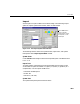
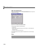
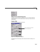

Table Of Contents
- Introduction
- LTI Models
- Operations on LTI Models
- Model Analysis Tools
- Arrays of LTI Models
- Customization
- Setting Toolbox Preferences
- Setting Tool Preferences
- Customizing Response Plot Properties
- Design Case Studies
- Reliable Computations
- GUI Reference
- SISO Design Tool Reference
- Menu Bar
- File
- Import
- Export
- Toolbox Preferences
- Print to Figure
- Close
- Edit
- Undo and Redo
- Root Locus and Bode Diagrams
- SISO Tool Preferences
- View
- Root Locus and Bode Diagrams
- System Data
- Closed Loop Poles
- Design History
- Tools
- Loop Responses
- Continuous/Discrete Conversions
- Draw a Simulink Diagram
- Compensator
- Format
- Edit
- Store
- Retrieve
- Clear
- Window
- Help
- Tool Bar
- Current Compensator
- Feedback Structure
- Root Locus Right-Click Menus
- Bode Diagram Right-Click Menus
- Status Panel
- Menu Bar
- LTI Viewer Reference
- Right-Click Menus for Response Plots
- Function Reference
- Functions by Category
- acker
- allmargin
- append
- augstate
- balreal
- bode
- bodemag
- c2d
- canon
- care
- chgunits
- connect
- covar
- ctrb
- ctrbf
- d2c
- d2d
- damp
- dare
- dcgain
- delay2z
- dlqr
- dlyap
- drss
- dsort
- dss
- dssdata
- esort
- estim
- evalfr
- feedback
- filt
- frd
- frdata
- freqresp
- gensig
- get
- gram
- hasdelay
- impulse
- initial
- interp
- inv
- isct, isdt
- isempty
- isproper
- issiso
- kalman
- kalmd
- lft
- lqgreg
- lqr
- lqrd
- lqry
- lsim
- ltimodels
- ltiprops
- ltiview
- lyap
- margin
- minreal
- modred
- ndims
- ngrid
- nichols
- norm
- nyquist
- obsv
- obsvf
- ord2
- pade
- parallel
- place
- pole
- pzmap
- reg
- reshape
- rlocus
- rss
- series
- set
- sgrid
- sigma
- sisotool
- size
- sminreal
- ss
- ss2ss
- ssbal
- ssdata
- stack
- step
- tf
- tfdata
- totaldelay
- zero
- zgrid
- zpk
- zpkdata
- Index
Menu Bar
13-13
•Open-Loop Nyquist — The open-loop Nyquist plot for your system
•
Open-Loop Nichols — The open-loop Nichols plot for your system
Customizing Loop Responses
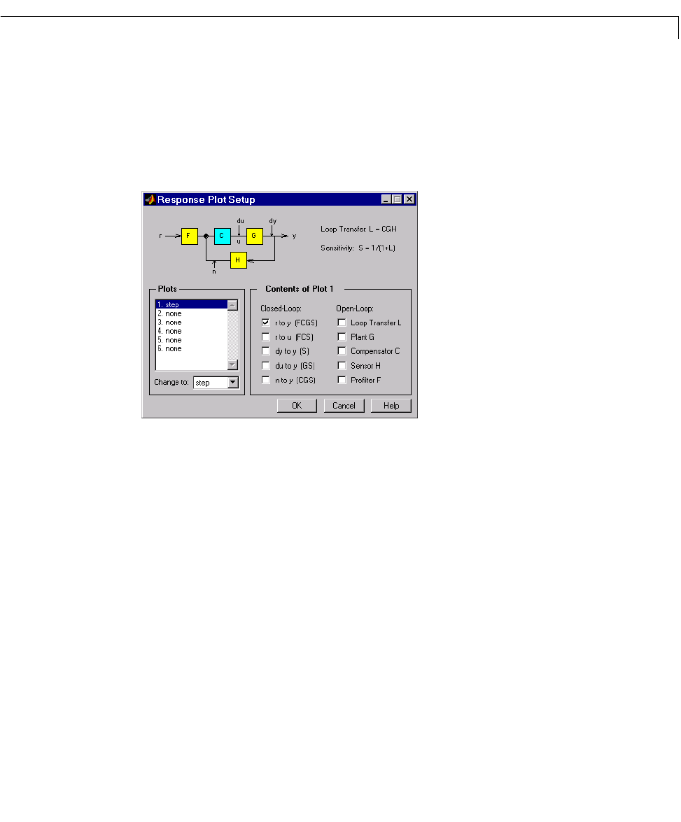
If you choose Custom from the list of loop responses, the Response Plot Setup
window opens.
Figure 13-7: Response Plot Setup Window
This window has many options for creating more specialized response plots,
but to use it properly you should be familiar with the basic features of the LTI
Viewer. If you are not, see Analyzing Models in GettingStartedwiththe
Control System Toolbox or “LTI Viewer” in the online documentation.
Loop diagram. At the top of the Response Plod Setup window is a loop diagram.
This block diagram shows the feedback structure of your system. The diagram
in Figure 13-7 shows the default configuration; the compensator is in the
forward path. If your system has the compensator in the feedback path, this
window correctly displays the alternate feedback structure.
The loop block diagram shows the arrangement of the components of your
system and the input/output structure. When selecting open- and closed-loop
responses in the Contents of Plots panel, refer to the loop diagram for
definitions of the responses.
Note that window lists two transfer functions next to the loop diagram: