
Specifications
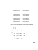
Table Of Contents
- Introduction
- LTI Models
- Operations on LTI Models
- Model Analysis Tools
- Arrays of LTI Models
- Customization
- Setting Toolbox Preferences
- Setting Tool Preferences
- Customizing Response Plot Properties
- Design Case Studies
- Reliable Computations
- GUI Reference
- SISO Design Tool Reference
- Menu Bar
- File
- Import
- Export
- Toolbox Preferences
- Print to Figure
- Close
- Edit
- Undo and Redo
- Root Locus and Bode Diagrams
- SISO Tool Preferences
- View
- Root Locus and Bode Diagrams
- System Data
- Closed Loop Poles
- Design History
- Tools
- Loop Responses
- Continuous/Discrete Conversions
- Draw a Simulink Diagram
- Compensator
- Format
- Edit
- Store
- Retrieve
- Clear
- Window
- Help
- Tool Bar
- Current Compensator
- Feedback Structure
- Root Locus Right-Click Menus
- Bode Diagram Right-Click Menus
- Status Panel
- Menu Bar
- LTI Viewer Reference
- Right-Click Menus for Response Plots
- Function Reference
- Functions by Category
- acker
- allmargin
- append
- augstate
- balreal
- bode
- bodemag
- c2d
- canon
- care
- chgunits
- connect
- covar
- ctrb
- ctrbf
- d2c
- d2d
- damp
- dare
- dcgain
- delay2z
- dlqr
- dlyap
- drss
- dsort
- dss
- dssdata
- esort
- estim
- evalfr
- feedback
- filt
- frd
- frdata
- freqresp
- gensig
- get
- gram
- hasdelay
- impulse
- initial
- interp
- inv
- isct, isdt
- isempty
- isproper
- issiso
- kalman
- kalmd
- lft
- lqgreg
- lqr
- lqrd
- lqry
- lsim
- ltimodels
- ltiprops
- ltiview
- lyap
- margin
- minreal
- modred
- ndims
- ngrid
- nichols
- norm
- nyquist
- obsv
- obsvf
- ord2
- pade
- parallel
- place
- pole
- pzmap
- reg
- reshape
- rlocus
- rss
- series
- set
- sgrid
- sigma
- sisotool
- size
- sminreal
- ss
- ss2ss
- ssbal
- ssdata
- stack
- step
- tf
- tfdata
- totaldelay
- zero
- zgrid
- zpk
- zpkdata
- Index

Choice of LTI Model
11-13
The condition number of the new eigenvector matrix
cond(vc)
ans =
34.5825
is thirty times larger.
The phenomenon illustrated aboveisnotunusual.Matrices in companionform
or controllable/observable canonical form (like
Ac) typically have
worse-conditioned eigensystems than matrices in general state-space form
(like
A). This means that their eigenvalues and eigenvectors are more sensitive
toperturbation.Theproblemgenerally getsfarworseforhigher-order systems.
Working with high-order transfer function models and converting them back
and forth to state space is numerically risky.
In summary, the main numerical problems to be aware of in dealing with
transfer function models (and hence, calculations involving polynomials) are:
•The potentially large range of numbers leads to ill-conditioned problems,
especially when such models are linked together giving high-order
polynomials.
•The pole locations are very sensitive to the coefficients of the denominator
polynomial.
•The balanced companion form produced by
ss, while better than the
standard companion form, often results in ill-conditioned eigenproblems,
especially with higher-order systems.
The above statements hold even for systems with distinct poles, but are
particularly relevant when poles are multiple.
Zero-Pole-Gain Models
The third major representation used for LTI models in MATLAB is the
factored, or zero-pole-gain (ZPK) representation. It is sometimes very
convenient to describe a model in this way although most major design
methodologies tend to be oriented towards either transfer functions or
state-space.
In contrast to polynomials, the ZPK representation of systems can be more
reliable. At the very least, the ZPK representation tends to avoid the