
Specifications

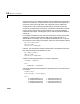
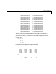
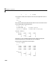
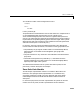
Table Of Contents
- Introduction
- LTI Models
- Operations on LTI Models
- Model Analysis Tools
- Arrays of LTI Models
- Customization
- Setting Toolbox Preferences
- Setting Tool Preferences
- Customizing Response Plot Properties
- Design Case Studies
- Reliable Computations
- GUI Reference
- SISO Design Tool Reference
- Menu Bar
- File
- Import
- Export
- Toolbox Preferences
- Print to Figure
- Close
- Edit
- Undo and Redo
- Root Locus and Bode Diagrams
- SISO Tool Preferences
- View
- Root Locus and Bode Diagrams
- System Data
- Closed Loop Poles
- Design History
- Tools
- Loop Responses
- Continuous/Discrete Conversions
- Draw a Simulink Diagram
- Compensator
- Format
- Edit
- Store
- Retrieve
- Clear
- Window
- Help
- Tool Bar
- Current Compensator
- Feedback Structure
- Root Locus Right-Click Menus
- Bode Diagram Right-Click Menus
- Status Panel
- Menu Bar
- LTI Viewer Reference
- Right-Click Menus for Response Plots
- Function Reference
- Functions by Category
- acker
- allmargin
- append
- augstate
- balreal
- bode
- bodemag
- c2d
- canon
- care
- chgunits
- connect
- covar
- ctrb
- ctrbf
- d2c
- d2d
- damp
- dare
- dcgain
- delay2z
- dlqr
- dlyap
- drss
- dsort
- dss
- dssdata
- esort
- estim
- evalfr
- feedback
- filt
- frd
- frdata
- freqresp
- gensig
- get
- gram
- hasdelay
- impulse
- initial
- interp
- inv
- isct, isdt
- isempty
- isproper
- issiso
- kalman
- kalmd
- lft
- lqgreg
- lqr
- lqrd
- lqry
- lsim
- ltimodels
- ltiprops
- ltiview
- lyap
- margin
- minreal
- modred
- ndims
- ngrid
- nichols
- norm
- nyquist
- obsv
- obsvf
- ord2
- pade
- parallel
- place
- pole
- pzmap
- reg
- reshape
- rlocus
- rss
- series
- set
- sgrid
- sigma
- sisotool
- size
- sminreal
- ss
- ss2ss
- ssbal
- ssdata
- stack
- step
- tf
- tfdata
- totaldelay
- zero
- zgrid
- zpk
- zpkdata
- Index

Choice of LTI Model
11-11
5.000000270433721e+00 5.000000000000000e+00
5.999998194359617e+00 6.000000000000000e+00
7.000004542844700e+00 7.000000000000000e+00
8.000013753274901e+00 8.000000000000000e+00
8.999848908317270e+00 9.000000000000000e+00
1.000059459550623e+01 1.000000000000000e+01
1.099854678336595e+01 1.100000000000000e+01
1.200255822210095e+01 1.200000000000000e+01
1.299647702454549e+01 1.300000000000000e+01
1.400406940833612e+01 1.400000000000000e+01
1.499604787386921e+01 1.500000000000000e+01
1.600304396718421e+01 1.600000000000000e+01
1.699828695210055e+01 1.700000000000000e+01
1.800062935148728e+01 1.800000000000000e+01
1.899986934359322e+01 1.900000000000000e+01
2.000001082693916e+01 2.000000000000000e+01
There is another difficulty with transfer function models when realized in
state-space form with
ss. They may give rise to badly conditioned eigenvector
matrices, even if the eigenvalues are well separated. For example, consider the
normal matrix
A = [5 4 1 1
4 5 1 1
1 1 4 2
1 1 2 4]
Its eigenvectors and eigenvalues are given as follows.
[v,d] = eig(A)
v =
0.7071 –0.0000 –0.3162 0.6325
–0.7071 0.0000 –0.3162 0.6325
0.0000 0.7071 0.6325 0.3162
–0.0000 –0.7071 0.6325 0.3162
d =
1.0000 0 0 0
0 2.0000 0 0
0 0 5.0000 0