
Specifications
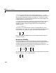
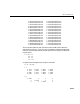
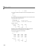
Table Of Contents
- Introduction
- LTI Models
- Operations on LTI Models
- Model Analysis Tools
- Arrays of LTI Models
- Customization
- Setting Toolbox Preferences
- Setting Tool Preferences
- Customizing Response Plot Properties
- Design Case Studies
- Reliable Computations
- GUI Reference
- SISO Design Tool Reference
- Menu Bar
- File
- Import
- Export
- Toolbox Preferences
- Print to Figure
- Close
- Edit
- Undo and Redo
- Root Locus and Bode Diagrams
- SISO Tool Preferences
- View
- Root Locus and Bode Diagrams
- System Data
- Closed Loop Poles
- Design History
- Tools
- Loop Responses
- Continuous/Discrete Conversions
- Draw a Simulink Diagram
- Compensator
- Format
- Edit
- Store
- Retrieve
- Clear
- Window
- Help
- Tool Bar
- Current Compensator
- Feedback Structure
- Root Locus Right-Click Menus
- Bode Diagram Right-Click Menus
- Status Panel
- Menu Bar
- LTI Viewer Reference
- Right-Click Menus for Response Plots
- Function Reference
- Functions by Category
- acker
- allmargin
- append
- augstate
- balreal
- bode
- bodemag
- c2d
- canon
- care
- chgunits
- connect
- covar
- ctrb
- ctrbf
- d2c
- d2d
- damp
- dare
- dcgain
- delay2z
- dlqr
- dlyap
- drss
- dsort
- dss
- dssdata
- esort
- estim
- evalfr
- feedback
- filt
- frd
- frdata
- freqresp
- gensig
- get
- gram
- hasdelay
- impulse
- initial
- interp
- inv
- isct, isdt
- isempty
- isproper
- issiso
- kalman
- kalmd
- lft
- lqgreg
- lqr
- lqrd
- lqry
- lsim
- ltimodels
- ltiprops
- ltiview
- lyap
- margin
- minreal
- modred
- ndims
- ngrid
- nichols
- norm
- nyquist
- obsv
- obsvf
- ord2
- pade
- parallel
- place
- pole
- pzmap
- reg
- reshape
- rlocus
- rss
- series
- set
- sgrid
- sigma
- sisotool
- size
- sminreal
- ss
- ss2ss
- ssbal
- ssdata
- stack
- step
- tf
- tfdata
- totaldelay
- zero
- zgrid
- zpk
- zpkdata
- Index

11 Reliable Computations
11-10
very little. This is true ingeneral. Different roots have different sensitivities to
different perturbations. Computed roots may then be quite meaningless for a
polynomial, particularly high-order, with imprecisely known coefficients.
Finding all the roots of a polynomial (equivalently, the poles of a transfer
function or the eigenvalues of a matrix in controllable or observable canonical
form) is often an intrinsically sensitive problem. For a clear and detailed
treatment of the subject, including the tricky numerical problem of deflation,
consult [6].
It is therefore preferable to work with the factored form of polynomials when
available. To compute a state-space model of the transfer function
defined above, for example, you could expand the denominator of , convert
the transfer function model to state space, and extract the state-space data by
H1 = tf(1,poly(1:20))
H1ss = ss(H1)
[a1,b1,c1] = ssdata(H1)
However, you should rather keep the denominator in factored form and work
with the zero-pole-gain representation of .
H2 = zpk([],1:20,1)
H2ss = ss(H2)
[a2,b2,c2] = ssdata(H2)
Indeed, the resulting state matrix a2 is better conditioned.
[cond(a1) cond(a2)]
ans =
2.7681e+03 8.8753e+01
and the conversion from zero-pole-gain to state space incurs no loss of accuracy
in the poles.
format long e
[sort(eig(a1)) sort(eig(a2))]
ans =
9.999999999998792e-01 1.000000000000000e+00
2.000000000001984e+00 2.000000000000000e+00
3.000000000475623e+00 3.000000000000000e+00
3.999999981263996e+00 4.000000000000000e+00
Hs
()
H
Hs
()