
Specifications

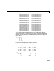

Table Of Contents
- Introduction
- LTI Models
- Operations on LTI Models
- Model Analysis Tools
- Arrays of LTI Models
- Customization
- Setting Toolbox Preferences
- Setting Tool Preferences
- Customizing Response Plot Properties
- Design Case Studies
- Reliable Computations
- GUI Reference
- SISO Design Tool Reference
- Menu Bar
- File
- Import
- Export
- Toolbox Preferences
- Print to Figure
- Close
- Edit
- Undo and Redo
- Root Locus and Bode Diagrams
- SISO Tool Preferences
- View
- Root Locus and Bode Diagrams
- System Data
- Closed Loop Poles
- Design History
- Tools
- Loop Responses
- Continuous/Discrete Conversions
- Draw a Simulink Diagram
- Compensator
- Format
- Edit
- Store
- Retrieve
- Clear
- Window
- Help
- Tool Bar
- Current Compensator
- Feedback Structure
- Root Locus Right-Click Menus
- Bode Diagram Right-Click Menus
- Status Panel
- Menu Bar
- LTI Viewer Reference
- Right-Click Menus for Response Plots
- Function Reference
- Functions by Category
- acker
- allmargin
- append
- augstate
- balreal
- bode
- bodemag
- c2d
- canon
- care
- chgunits
- connect
- covar
- ctrb
- ctrbf
- d2c
- d2d
- damp
- dare
- dcgain
- delay2z
- dlqr
- dlyap
- drss
- dsort
- dss
- dssdata
- esort
- estim
- evalfr
- feedback
- filt
- frd
- frdata
- freqresp
- gensig
- get
- gram
- hasdelay
- impulse
- initial
- interp
- inv
- isct, isdt
- isempty
- isproper
- issiso
- kalman
- kalmd
- lft
- lqgreg
- lqr
- lqrd
- lqry
- lsim
- ltimodels
- ltiprops
- ltiview
- lyap
- margin
- minreal
- modred
- ndims
- ngrid
- nichols
- norm
- nyquist
- obsv
- obsvf
- ord2
- pade
- parallel
- place
- pole
- pzmap
- reg
- reshape
- rlocus
- rss
- series
- set
- sgrid
- sigma
- sisotool
- size
- sminreal
- ss
- ss2ss
- ssbal
- ssdata
- stack
- step
- tf
- tfdata
- totaldelay
- zero
- zgrid
- zpk
- zpkdata
- Index

Choice of LTI Model
11-9
A major difficulty is the extreme sensitivity of the roots of a polynomial to its
coefficients. This example is adapted from Wilkinson, [6] as an illustration.
Consider the transfer function
The matrix of the companion realization of is
Despite the benign looking poles of the system (at –1,–2,..., –20) you are faced
with a rather large range in the elements of , from 1 to . But
the difficulties don’t stop here. Suppose the coefficient of in the transfer
function (or ) is perturbed from 210 to ( ).
Then, computed on a VAX (IEEE arithmetic has enough mantissa for only
), the poles of the perturbed transfer function (equivalently, the
eigenvalues of ) are
eig(A)'
ans =
Columns 1 through 7
–19.9998 –19.0019 –17.9916 –17.0217 –15.9594 –15.0516 –13.9504
Columns 8 through 14
–13.0369 –11.9805 –11.0081 –9.9976 –9.0005 –7.9999 –7.0000
Columns 15 through 20
–6.0000 –5.0000 –4.0000 –3.0000 –2.0000 –1.0000
The problem here is not roundoff. Rather, high-order polynomials are simply
intrinsically very sensitive, even when the zeros are well separated. In this
case, a relative perturbation of the order of induced relative
perturbationsof the order of in some roots. But some of the roots changed
Hs
()
1
s 1+
()
s 2+
()
... s 20+
()
-------------------------------------------------------------
1
s
20
210s
19
... 20!+++
-----------------------------------------------------------
==
AHs
()
A
0 1 0 ... 0
0 0 1 ... 0
::..:
0 0 ... . 1
20!– . ... . 210–
=
A 20! 2.4 10
18
×≈
s
19
Ann
,()
210 2
23–
+ 2
23–
1.2 10
7–
×≈
n 17=
A
10
9–
10
2–