
Specifications
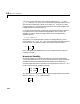

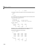
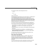

Table Of Contents
- Introduction
- LTI Models
- Operations on LTI Models
- Model Analysis Tools
- Arrays of LTI Models
- Customization
- Setting Toolbox Preferences
- Setting Tool Preferences
- Customizing Response Plot Properties
- Design Case Studies
- Reliable Computations
- GUI Reference
- SISO Design Tool Reference
- Menu Bar
- File
- Import
- Export
- Toolbox Preferences
- Print to Figure
- Close
- Edit
- Undo and Redo
- Root Locus and Bode Diagrams
- SISO Tool Preferences
- View
- Root Locus and Bode Diagrams
- System Data
- Closed Loop Poles
- Design History
- Tools
- Loop Responses
- Continuous/Discrete Conversions
- Draw a Simulink Diagram
- Compensator
- Format
- Edit
- Store
- Retrieve
- Clear
- Window
- Help
- Tool Bar
- Current Compensator
- Feedback Structure
- Root Locus Right-Click Menus
- Bode Diagram Right-Click Menus
- Status Panel
- Menu Bar
- LTI Viewer Reference
- Right-Click Menus for Response Plots
- Function Reference
- Functions by Category
- acker
- allmargin
- append
- augstate
- balreal
- bode
- bodemag
- c2d
- canon
- care
- chgunits
- connect
- covar
- ctrb
- ctrbf
- d2c
- d2d
- damp
- dare
- dcgain
- delay2z
- dlqr
- dlyap
- drss
- dsort
- dss
- dssdata
- esort
- estim
- evalfr
- feedback
- filt
- frd
- frdata
- freqresp
- gensig
- get
- gram
- hasdelay
- impulse
- initial
- interp
- inv
- isct, isdt
- isempty
- isproper
- issiso
- kalman
- kalmd
- lft
- lqgreg
- lqr
- lqrd
- lqry
- lsim
- ltimodels
- ltiprops
- ltiview
- lyap
- margin
- minreal
- modred
- ndims
- ngrid
- nichols
- norm
- nyquist
- obsv
- obsvf
- ord2
- pade
- parallel
- place
- pole
- pzmap
- reg
- reshape
- rlocus
- rss
- series
- set
- sgrid
- sigma
- sisotool
- size
- sminreal
- ss
- ss2ss
- ssbal
- ssdata
- stack
- step
- tf
- tfdata
- totaldelay
- zero
- zgrid
- zpk
- zpkdata
- Index

11 Reliable Computations
11-6
row of A. This perturbed matrix has n distinct eigenvalues with
. Thus, you can see that this small perturbation in the
data has been magnified by a factor on the order of to result in a rather
large perturbation in the solution (the eigenvalues of
A). Further details and
relatedexamplesaretobefoundin[7].
It is important to realize that a matrix can be ill-conditioned with respect to
inversion but have a well-conditioned eigenproblem, and vice versa. For
example, consider an upper triangular matrix of ones (zeros below the
diagonal) given by
A = triu(ones(n));
This matrix is ill-conditioned with respect to its eigenproblem (try small
perturbations in
A(n,1) for, say, n=20), but is well-conditioned with respect to
inversion (check its condition number). On the other hand, the matrix
has a well-conditioned eigenproblem, but is ill-conditioned with respect to
inversion for small .
Numerical Stability
Numerical stability is somewhat more difficult to illustrate meaningfully.
Consult the references in [5], [6], and [7] for further details. Here is one small
example to illustrate the difference between stability and conditioning.
Gaussian elimination with no pivoting for solving the linear system is
known to be numerically unstable. Consider
Allcomputationsarecarriedoutinthree-significant-figuredecimalarithmetic.
Thetrueanswer isapproximately
λ
1
...
λ
n
,,
λ
k
12
⁄
j2
π
kn
⁄()
exp=
2
n
A
11
11
δ
+
=
δ
Ax b=
A
0.001 1.000
1.000 1.000–
= b
1.000
0.000
=
xA
1–
b=
x
0.999
0.999
=