
Specifications
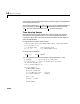
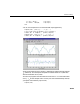


Table Of Contents
- Introduction
- LTI Models
- Operations on LTI Models
- Model Analysis Tools
- Arrays of LTI Models
- Customization
- Setting Toolbox Preferences
- Setting Tool Preferences
- Customizing Response Plot Properties
- Design Case Studies
- Reliable Computations
- GUI Reference
- SISO Design Tool Reference
- Menu Bar
- File
- Import
- Export
- Toolbox Preferences
- Print to Figure
- Close
- Edit
- Undo and Redo
- Root Locus and Bode Diagrams
- SISO Tool Preferences
- View
- Root Locus and Bode Diagrams
- System Data
- Closed Loop Poles
- Design History
- Tools
- Loop Responses
- Continuous/Discrete Conversions
- Draw a Simulink Diagram
- Compensator
- Format
- Edit
- Store
- Retrieve
- Clear
- Window
- Help
- Tool Bar
- Current Compensator
- Feedback Structure
- Root Locus Right-Click Menus
- Bode Diagram Right-Click Menus
- Status Panel
- Menu Bar
- LTI Viewer Reference
- Right-Click Menus for Response Plots
- Function Reference
- Functions by Category
- acker
- allmargin
- append
- augstate
- balreal
- bode
- bodemag
- c2d
- canon
- care
- chgunits
- connect
- covar
- ctrb
- ctrbf
- d2c
- d2d
- damp
- dare
- dcgain
- delay2z
- dlqr
- dlyap
- drss
- dsort
- dss
- dssdata
- esort
- estim
- evalfr
- feedback
- filt
- frd
- frdata
- freqresp
- gensig
- get
- gram
- hasdelay
- impulse
- initial
- interp
- inv
- isct, isdt
- isempty
- isproper
- issiso
- kalman
- kalmd
- lft
- lqgreg
- lqr
- lqrd
- lqry
- lsim
- ltimodels
- ltiprops
- ltiview
- lyap
- margin
- minreal
- modred
- ndims
- ngrid
- nichols
- norm
- nyquist
- obsv
- obsvf
- ord2
- pade
- parallel
- place
- pole
- pzmap
- reg
- reshape
- rlocus
- rss
- series
- set
- sgrid
- sigma
- sisotool
- size
- sminreal
- ss
- ss2ss
- ssbal
- ssdata
- stack
- step
- tf
- tfdata
- totaldelay
- zero
- zgrid
- zpk
- zpkdata
- Index

10 Design Case Studies
10-58
For simplicity, we have dropped the subscripts indicating the time dependence
of the state-space matrices.
Given initial conditions and , you can iterate these equations to
perform the filtering. Note that you must update both the state estimates
and error covariance matrices at each time sample.
Time-Varying Design
Although the Control System Toolbox does not offer specific commands to
perform time-varying Kalman filtering, it is easy to implement the filter
recursions in MATLAB. This section shows how to do this for the stationary
plant considered above.
First generate noisy output measurements
% Use process noise w and measurement noise v generated above
sys = ss(A,B,C,0,-1);
y = lsim(sys,u+w); % w = process noise
yv = y + v; % v = measurement noise
Given the initial conditions
you can implement the time-varying filter with the following
for loop.
P = B*Q*B'; % Initial error covariance
x = zeros(3,1); % Initial condition on the state
ye = zeros(length(t),1);
ycov = zeros(length(t),1);
for i=1:length(t)
% Measurement update
Mn = P*C'/(C*P*C'+R);
x = x + Mn*(yv(i)-C*x); % x[n|n]
P = (eye(3)-Mn*C)*P; % P[n|n]
ye(i) = C*x;
errcov(i) = C*P*C';
% Time update
x 10
[]
P 10
[]
xn.
[]
Pn.
[]
x 10
[]
0,= P 10
[]
BQB
T
=