
Specifications

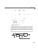
Table Of Contents
- Introduction
- LTI Models
- Operations on LTI Models
- Model Analysis Tools
- Arrays of LTI Models
- Customization
- Setting Toolbox Preferences
- Setting Tool Preferences
- Customizing Response Plot Properties
- Design Case Studies
- Reliable Computations
- GUI Reference
- SISO Design Tool Reference
- Menu Bar
- File
- Import
- Export
- Toolbox Preferences
- Print to Figure
- Close
- Edit
- Undo and Redo
- Root Locus and Bode Diagrams
- SISO Tool Preferences
- View
- Root Locus and Bode Diagrams
- System Data
- Closed Loop Poles
- Design History
- Tools
- Loop Responses
- Continuous/Discrete Conversions
- Draw a Simulink Diagram
- Compensator
- Format
- Edit
- Store
- Retrieve
- Clear
- Window
- Help
- Tool Bar
- Current Compensator
- Feedback Structure
- Root Locus Right-Click Menus
- Bode Diagram Right-Click Menus
- Status Panel
- Menu Bar
- LTI Viewer Reference
- Right-Click Menus for Response Plots
- Function Reference
- Functions by Category
- acker
- allmargin
- append
- augstate
- balreal
- bode
- bodemag
- c2d
- canon
- care
- chgunits
- connect
- covar
- ctrb
- ctrbf
- d2c
- d2d
- damp
- dare
- dcgain
- delay2z
- dlqr
- dlyap
- drss
- dsort
- dss
- dssdata
- esort
- estim
- evalfr
- feedback
- filt
- frd
- frdata
- freqresp
- gensig
- get
- gram
- hasdelay
- impulse
- initial
- interp
- inv
- isct, isdt
- isempty
- isproper
- issiso
- kalman
- kalmd
- lft
- lqgreg
- lqr
- lqrd
- lqry
- lsim
- ltimodels
- ltiprops
- ltiview
- lyap
- margin
- minreal
- modred
- ndims
- ngrid
- nichols
- norm
- nyquist
- obsv
- obsvf
- ord2
- pade
- parallel
- place
- pole
- pzmap
- reg
- reshape
- rlocus
- rss
- series
- set
- sgrid
- sigma
- sisotool
- size
- sminreal
- ss
- ss2ss
- ssbal
- ssdata
- stack
- step
- tf
- tfdata
- totaldelay
- zero
- zgrid
- zpk
- zpkdata
- Index

10 Design Case Studies
10-50
Kalman Filtering
This final case study illustrates the use of the Control System Toolbox for
Kalman filter design and simulation. Both steady-state and time-varying
Kalman filters are considered.
Consider the discrete plant
with additive Gaussian noise on the input and data
A = [1.1269 -0.4940 0.1129
1.0000 0 0
0 1.0000 0];
B = [-0.3832
0.5919
0.5191];
C = [1 0 0];
Our goal is to design a Kalman filter that estimates the output given the
inputs and the noisy output measurements
where is some Gaussian white noise.
Discrete Kalman Filter
The equations of the steady-state Kalman filter for this problem are given as
follows.
Measurement update
Time update
xn 1+
[]
Ax n
[]
Bun
[]
wn
[]
+
()
+=
yn
[]
Cx n
[]
=
wn
[]
un
[]
yn
[]
un
[]
y
v
n
[]
Cx n
[]
vn
[]
+=
vn
[]
x
ˆ
nn
[]
x
ˆ
nn 1–
[]
My
v
n
[]
Cx
ˆ
nn 1–
[]
–
()
+=
x
ˆ
n 1 n+[]Ax
ˆ
nn[]Bu n[]+=