
Specifications


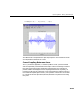
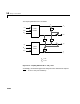
Table Of Contents
- Introduction
- LTI Models
- Operations on LTI Models
- Model Analysis Tools
- Arrays of LTI Models
- Customization
- Setting Toolbox Preferences
- Setting Tool Preferences
- Customizing Response Plot Properties
- Design Case Studies
- Reliable Computations
- GUI Reference
- SISO Design Tool Reference
- Menu Bar
- File
- Import
- Export
- Toolbox Preferences
- Print to Figure
- Close
- Edit
- Undo and Redo
- Root Locus and Bode Diagrams
- SISO Tool Preferences
- View
- Root Locus and Bode Diagrams
- System Data
- Closed Loop Poles
- Design History
- Tools
- Loop Responses
- Continuous/Discrete Conversions
- Draw a Simulink Diagram
- Compensator
- Format
- Edit
- Store
- Retrieve
- Clear
- Window
- Help
- Tool Bar
- Current Compensator
- Feedback Structure
- Root Locus Right-Click Menus
- Bode Diagram Right-Click Menus
- Status Panel
- Menu Bar
- LTI Viewer Reference
- Right-Click Menus for Response Plots
- Function Reference
- Functions by Category
- acker
- allmargin
- append
- augstate
- balreal
- bode
- bodemag
- c2d
- canon
- care
- chgunits
- connect
- covar
- ctrb
- ctrbf
- d2c
- d2d
- damp
- dare
- dcgain
- delay2z
- dlqr
- dlyap
- drss
- dsort
- dss
- dssdata
- esort
- estim
- evalfr
- feedback
- filt
- frd
- frdata
- freqresp
- gensig
- get
- gram
- hasdelay
- impulse
- initial
- interp
- inv
- isct, isdt
- isempty
- isproper
- issiso
- kalman
- kalmd
- lft
- lqgreg
- lqr
- lqrd
- lqry
- lsim
- ltimodels
- ltiprops
- ltiview
- lyap
- margin
- minreal
- modred
- ndims
- ngrid
- nichols
- norm
- nyquist
- obsv
- obsvf
- ord2
- pade
- parallel
- place
- pole
- pzmap
- reg
- reshape
- rlocus
- rss
- series
- set
- sgrid
- sigma
- sisotool
- size
- sminreal
- ss
- ss2ss
- ssbal
- ssdata
- stack
- step
- tf
- tfdata
- totaldelay
- zero
- zgrid
- zpk
- zpkdata
- Index

LQG Regulation: Rolling Mill Example
10-45
Let’s see how the previous “decoupled” LQG design fares when cross-coupling
is taken into account. To build the two-axes model shown in Figure 10-2,
append the models
Px and Py for the - and -axes.
P = append(Px,Py)
For convenience, reorder the inputs and outputs so that the commands and
thickness gaps appear first.
P = P([1 3 2 4],[1 4 2 3 5 6])
P.outputname
ans =
'x-gap'
'y-gap'
'x-force'
'y-force'
Finally, place the cross-coupling matrix in series with the outputs.
gxy = 0.1; gyx = 0.4;
CCmat = [eye(2) [0 gyx*gx;gxy*gy 0] ; zeros(2) [1 -gyx;-gxy 1]]
Pc = CCmat * P
Pc.outputname = P.outputname
To simulate the closed-loop response, also form the closed-loop model by
feedin = 1:2 % first two inputs of Pc are the commands
feedout = 3:4 % last two outputs of Pc are the measurements
cl = feedback(Pc,append(Regx,Regy),feedin,feedout,+1)
You are now ready to simulate the open- and closed-loop responses to the
driving white noises
wx (for the -axis) and wy (for the -axis).
wxy = [wx ; wy]
δ
x
δ
y
f
x
f
y
100g
yx
g
x
01g
xy
g
y
0
001g
yx
–
00g
xy
– 1
δ
x
δ
y
f
x
f
y
=
cross-coupling matrix
ì
x
y
x
y