
Specifications
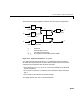
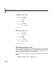
Table Of Contents
- Introduction
- LTI Models
- Operations on LTI Models
- Model Analysis Tools
- Arrays of LTI Models
- Customization
- Setting Toolbox Preferences
- Setting Tool Preferences
- Customizing Response Plot Properties
- Design Case Studies
- Reliable Computations
- GUI Reference
- SISO Design Tool Reference
- Menu Bar
- File
- Import
- Export
- Toolbox Preferences
- Print to Figure
- Close
- Edit
- Undo and Redo
- Root Locus and Bode Diagrams
- SISO Tool Preferences
- View
- Root Locus and Bode Diagrams
- System Data
- Closed Loop Poles
- Design History
- Tools
- Loop Responses
- Continuous/Discrete Conversions
- Draw a Simulink Diagram
- Compensator
- Format
- Edit
- Store
- Retrieve
- Clear
- Window
- Help
- Tool Bar
- Current Compensator
- Feedback Structure
- Root Locus Right-Click Menus
- Bode Diagram Right-Click Menus
- Status Panel
- Menu Bar
- LTI Viewer Reference
- Right-Click Menus for Response Plots
- Function Reference
- Functions by Category
- acker
- allmargin
- append
- augstate
- balreal
- bode
- bodemag
- c2d
- canon
- care
- chgunits
- connect
- covar
- ctrb
- ctrbf
- d2c
- d2d
- damp
- dare
- dcgain
- delay2z
- dlqr
- dlyap
- drss
- dsort
- dss
- dssdata
- esort
- estim
- evalfr
- feedback
- filt
- frd
- frdata
- freqresp
- gensig
- get
- gram
- hasdelay
- impulse
- initial
- interp
- inv
- isct, isdt
- isempty
- isproper
- issiso
- kalman
- kalmd
- lft
- lqgreg
- lqr
- lqrd
- lqry
- lsim
- ltimodels
- ltiprops
- ltiview
- lyap
- margin
- minreal
- modred
- ndims
- ngrid
- nichols
- norm
- nyquist
- obsv
- obsvf
- ord2
- pade
- parallel
- place
- pole
- pzmap
- reg
- reshape
- rlocus
- rss
- series
- set
- sgrid
- sigma
- sisotool
- size
- sminreal
- ss
- ss2ss
- ssbal
- ssdata
- stack
- step
- tf
- tfdata
- totaldelay
- zero
- zgrid
- zpk
- zpkdata
- Index

10 Design Case Studies
10-36
ans =
'x-gap'
'x-force'
The second output 'x-force' is the rolling force measurement. The LQG
regulator willusethismeasurement to drive thehydraulic actuatorandreduce
disturbance-induced thickness variations .
The LQG design involves two steps:
1 Design a full-state-feedback gain that minimizes an LQ performance
measure of the form
2 Design a Kalman filter that estimates the state vector given the force
measurements
'x-force'.
The performance criterion penalizes low and high frequencies equally.
Because low-frequency variations are of primary concern, eliminate the
high-frequency content of with the low-pass filter and use the
filtered value in the LQ performance criterion.
lpf = tf(30,[1 30])
% Connect low-pass filter to first output of Px
Pxdes = append(lpf,1) * Px
set(Pxdes,'outputn',{'x-gap*' 'x-force'})
% Design the state-feedback gain using LQRY and q=1, r=1e-4
kx = lqry(Pxdes(1,1),1,1e-4)
δ
x
Ju
x
()
q
δ
x
2
ru
x
2
+
îþ
td
0
∞
ò
=
Ju
x
()
δ
x
30 s 30+
()⁄