
Specifications

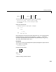
Table Of Contents
- Introduction
- LTI Models
- Operations on LTI Models
- Model Analysis Tools
- Arrays of LTI Models
- Customization
- Setting Toolbox Preferences
- Setting Tool Preferences
- Customizing Response Plot Properties
- Design Case Studies
- Reliable Computations
- GUI Reference
- SISO Design Tool Reference
- Menu Bar
- File
- Import
- Export
- Toolbox Preferences
- Print to Figure
- Close
- Edit
- Undo and Redo
- Root Locus and Bode Diagrams
- SISO Tool Preferences
- View
- Root Locus and Bode Diagrams
- System Data
- Closed Loop Poles
- Design History
- Tools
- Loop Responses
- Continuous/Discrete Conversions
- Draw a Simulink Diagram
- Compensator
- Format
- Edit
- Store
- Retrieve
- Clear
- Window
- Help
- Tool Bar
- Current Compensator
- Feedback Structure
- Root Locus Right-Click Menus
- Bode Diagram Right-Click Menus
- Status Panel
- Menu Bar
- LTI Viewer Reference
- Right-Click Menus for Response Plots
- Function Reference
- Functions by Category
- acker
- allmargin
- append
- augstate
- balreal
- bode
- bodemag
- c2d
- canon
- care
- chgunits
- connect
- covar
- ctrb
- ctrbf
- d2c
- d2d
- damp
- dare
- dcgain
- delay2z
- dlqr
- dlyap
- drss
- dsort
- dss
- dssdata
- esort
- estim
- evalfr
- feedback
- filt
- frd
- frdata
- freqresp
- gensig
- get
- gram
- hasdelay
- impulse
- initial
- interp
- inv
- isct, isdt
- isempty
- isproper
- issiso
- kalman
- kalmd
- lft
- lqgreg
- lqr
- lqrd
- lqry
- lsim
- ltimodels
- ltiprops
- ltiview
- lyap
- margin
- minreal
- modred
- ndims
- ngrid
- nichols
- norm
- nyquist
- obsv
- obsvf
- ord2
- pade
- parallel
- place
- pole
- pzmap
- reg
- reshape
- rlocus
- rss
- series
- set
- sgrid
- sigma
- sisotool
- size
- sminreal
- ss
- ss2ss
- ssbal
- ssdata
- stack
- step
- tf
- tfdata
- totaldelay
- zero
- zgrid
- zpk
- zpkdata
- Index

2 LTI Models
2-4
Creating an LTI Object: An Example
An LTI object of the type TF, ZPK, SS, or FRD is created whenever you invoke
the corresponding constructor function,
tf, zpk, ss,orfrd. For example,
P = tf([1 2],[1 1 10])
creates a TF object, P, that stores the numerator and denominator coefficients
of the transfer function
See “Creating LTI Models” on page 2-8 for methods for creating all of the LTI
object types.
LTI Properties and Methods
The LTI object implementation relies on MATLAB object-oriented
programming capabilities. Objects are MATLAB structures with an additional
flag indicating their class (TF, ZPK, SS, or FRD for LTI objects) and have
pre-defined fields called object properties. For LTI objects, these properties
include the model data, sample time, delay times, input or output names, and
input or output groups (see “LTI Properties” on page 2-25 for details). The
functions that operate on a particular object are called the object methods.
These may include customized versions of simple operations such as addition
or multiplication. For example,
P = tf([1 2],[1 1 10])
Q = 2 + P
performs transfer function addition.
The object-specific versions of such standard operations are called overloaded
operations. For more details on objects, methods, and object-oriented
programming, see Chapter 14, “Classes and Objects” in Using MATLAB.For
details on operations on LTI objects, see Chapter 3, “Operations on LTI
Models.”
Ps
()
s 2+
s
2
s 10++
---------------------------
=
Qs
()
2 Ps
()
+
2s
2
3s 22++
s
2
s 10++
-----------------------------------
==