
Specifications


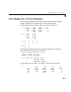
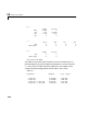
Table Of Contents
- Introduction
- LTI Models
- Operations on LTI Models
- Model Analysis Tools
- Arrays of LTI Models
- Customization
- Setting Toolbox Preferences
- Setting Tool Preferences
- Customizing Response Plot Properties
- Design Case Studies
- Reliable Computations
- GUI Reference
- SISO Design Tool Reference
- Menu Bar
- File
- Import
- Export
- Toolbox Preferences
- Print to Figure
- Close
- Edit
- Undo and Redo
- Root Locus and Bode Diagrams
- SISO Tool Preferences
- View
- Root Locus and Bode Diagrams
- System Data
- Closed Loop Poles
- Design History
- Tools
- Loop Responses
- Continuous/Discrete Conversions
- Draw a Simulink Diagram
- Compensator
- Format
- Edit
- Store
- Retrieve
- Clear
- Window
- Help
- Tool Bar
- Current Compensator
- Feedback Structure
- Root Locus Right-Click Menus
- Bode Diagram Right-Click Menus
- Status Panel
- Menu Bar
- LTI Viewer Reference
- Right-Click Menus for Response Plots
- Function Reference
- Functions by Category
- acker
- allmargin
- append
- augstate
- balreal
- bode
- bodemag
- c2d
- canon
- care
- chgunits
- connect
- covar
- ctrb
- ctrbf
- d2c
- d2d
- damp
- dare
- dcgain
- delay2z
- dlqr
- dlyap
- drss
- dsort
- dss
- dssdata
- esort
- estim
- evalfr
- feedback
- filt
- frd
- frdata
- freqresp
- gensig
- get
- gram
- hasdelay
- impulse
- initial
- interp
- inv
- isct, isdt
- isempty
- isproper
- issiso
- kalman
- kalmd
- lft
- lqgreg
- lqr
- lqrd
- lqry
- lsim
- ltimodels
- ltiprops
- ltiview
- lyap
- margin
- minreal
- modred
- ndims
- ngrid
- nichols
- norm
- nyquist
- obsv
- obsvf
- ord2
- pade
- parallel
- place
- pole
- pzmap
- reg
- reshape
- rlocus
- rss
- series
- set
- sgrid
- sigma
- sisotool
- size
- sminreal
- ss
- ss2ss
- ssbal
- ssdata
- stack
- step
- tf
- tfdata
- totaldelay
- zero
- zgrid
- zpk
- zpkdata
- Index

Yaw Damper for a 747 Jet Transport
10-3
Yaw Damper for a 747 Jet Transport
This case study demonstrates the tools for classical control design by stepping
through the design of a yaw damper for a 747 jet transport aircraft.
The jet model during cruise flight at MACH = 0.8 and H = 40,000 ft. is
A = [-0.0558 -0.9968 0.0802 0.0415
0.5980 -0.1150 -0.0318 0
-3.0500 0.3880 -0.4650 0
0 0.0805 1.0000 0];
B = [ 0.0729 0.0000
-4.7500 0.00775
.15300 0.1430
0 0];
C = [0 1 0 0
0 0 0 1];
D = [0 0
0 0];
The following commands specify this state-space model as an LTI object and
attach names to the states, inputs, and outputs.
states = {'beta' 'yaw' 'roll' 'phi'};
inputs = {'rudder' 'aileron'};
outputs = {'yaw' 'bank angle'};
sys = ss(A,B,C,D,'statename',states,...
'inputname',inputs,...
'outputname',outputs);
You can display the LTI model sys by typing sys.MATLABrespondswith
a =
beta yaw roll phi
beta -0.0558 -0.9968 0.0802 0.0415
yaw 0.598 -0.115 -0.0318 0
roll -3.05 0.388 -0.465 0
phi 0 0.0805 1 0