
Specifications
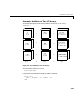
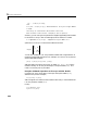
Table Of Contents
- Introduction
- LTI Models
- Operations on LTI Models
- Model Analysis Tools
- Arrays of LTI Models
- Customization
- Setting Toolbox Preferences
- Setting Tool Preferences
- Customizing Response Plot Properties
- Design Case Studies
- Reliable Computations
- GUI Reference
- SISO Design Tool Reference
- Menu Bar
- File
- Import
- Export
- Toolbox Preferences
- Print to Figure
- Close
- Edit
- Undo and Redo
- Root Locus and Bode Diagrams
- SISO Tool Preferences
- View
- Root Locus and Bode Diagrams
- System Data
- Closed Loop Poles
- Design History
- Tools
- Loop Responses
- Continuous/Discrete Conversions
- Draw a Simulink Diagram
- Compensator
- Format
- Edit
- Store
- Retrieve
- Clear
- Window
- Help
- Tool Bar
- Current Compensator
- Feedback Structure
- Root Locus Right-Click Menus
- Bode Diagram Right-Click Menus
- Status Panel
- Menu Bar
- LTI Viewer Reference
- Right-Click Menus for Response Plots
- Function Reference
- Functions by Category
- acker
- allmargin
- append
- augstate
- balreal
- bode
- bodemag
- c2d
- canon
- care
- chgunits
- connect
- covar
- ctrb
- ctrbf
- d2c
- d2d
- damp
- dare
- dcgain
- delay2z
- dlqr
- dlyap
- drss
- dsort
- dss
- dssdata
- esort
- estim
- evalfr
- feedback
- filt
- frd
- frdata
- freqresp
- gensig
- get
- gram
- hasdelay
- impulse
- initial
- interp
- inv
- isct, isdt
- isempty
- isproper
- issiso
- kalman
- kalmd
- lft
- lqgreg
- lqr
- lqrd
- lqry
- lsim
- ltimodels
- ltiprops
- ltiview
- lyap
- margin
- minreal
- modred
- ndims
- ngrid
- nichols
- norm
- nyquist
- obsv
- obsvf
- ord2
- pade
- parallel
- place
- pole
- pzmap
- reg
- reshape
- rlocus
- rss
- series
- set
- sgrid
- sigma
- sisotool
- size
- sminreal
- ss
- ss2ss
- ssbal
- ssdata
- stack
- step
- tf
- tfdata
- totaldelay
- zero
- zgrid
- zpk
- zpkdata
- Index

Operations on LTI Arrays
5-27
dimensions as sys1. You can use shortcuts for coding sysa = op(sys1,sys2)
in the following cases:
•For operations that apply to LTI arrays,
sys2 doesnothavetobeanarray.
It can be a single LTI model (or a gain matrix) whose I/O dimensions satisfy
the compatibility requirements for
op (with those of each of the models in
sys1).Inthiscase,op applies sys2 to each model in sys1,andthekth model
in
sys satisfies
sysa(:,:,k) = op(sys1(:,:,k),sys2)
•For arithmetic operations, such as +, *, /,and\, sys2 can be either a single
SISOmodel,oranLTIarrayofSISO models,evenwhen
sys1 isanLTIarray
of MIMO models. This special case relies on MATLAB’s scalar expansion
capabilities for arithmetic operations.
- When
sys2 is a single SISO LTI model (or a scalar gain), op applies sys2
to sys1 on an entry-by-entry basis. Theijth entryin the kth model insysa
satisfies
sysa(i,j,k) = op(sys1(i,j,k),sys2)
- When sys2 is an LTI array of SISO models (or a multidimensional array
of scalar gains),
op appliessys2 to sys1 onan entry-by-entry basis for each
model in
sysa.
sysa(i,j,k) = op(sys1(i,j,k),sys2(:,:,k))
Examples of Operations on LTI Arrays with Single LTI Models
Suppose you want to create an LTI array containing three models, where, for
in the set , each model has the form
You can do this efficiently by first setting up an LTI array
h containing the
SISO models and then using concatenation to form the LTI array
H of
MIMO LTI models , . To do this, type
tau = [1.1 1.2 1.3];
for i=1:3 % Form LTI array h of SISO models.
τ
1.1 1.2 1.3
,,{}
H
τ
s
(
)
H
τ
s
()
1
s
τ
+
-----------
0
1–
1
s
---
=
1 s τ+(
)
⁄
H
τ
s(
)
τ 1.1 1.2 1.3,,{}∈