
Specifications
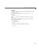

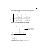
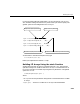
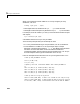
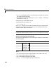
Table Of Contents
- Introduction
- LTI Models
- Operations on LTI Models
- Model Analysis Tools
- Arrays of LTI Models
- Customization
- Setting Toolbox Preferences
- Setting Tool Preferences
- Customizing Response Plot Properties
- Design Case Studies
- Reliable Computations
- GUI Reference
- SISO Design Tool Reference
- Menu Bar
- File
- Import
- Export
- Toolbox Preferences
- Print to Figure
- Close
- Edit
- Undo and Redo
- Root Locus and Bode Diagrams
- SISO Tool Preferences
- View
- Root Locus and Bode Diagrams
- System Data
- Closed Loop Poles
- Design History
- Tools
- Loop Responses
- Continuous/Discrete Conversions
- Draw a Simulink Diagram
- Compensator
- Format
- Edit
- Store
- Retrieve
- Clear
- Window
- Help
- Tool Bar
- Current Compensator
- Feedback Structure
- Root Locus Right-Click Menus
- Bode Diagram Right-Click Menus
- Status Panel
- Menu Bar
- LTI Viewer Reference
- Right-Click Menus for Response Plots
- Function Reference
- Functions by Category
- acker
- allmargin
- append
- augstate
- balreal
- bode
- bodemag
- c2d
- canon
- care
- chgunits
- connect
- covar
- ctrb
- ctrbf
- d2c
- d2d
- damp
- dare
- dcgain
- delay2z
- dlqr
- dlyap
- drss
- dsort
- dss
- dssdata
- esort
- estim
- evalfr
- feedback
- filt
- frd
- frdata
- freqresp
- gensig
- get
- gram
- hasdelay
- impulse
- initial
- interp
- inv
- isct, isdt
- isempty
- isproper
- issiso
- kalman
- kalmd
- lft
- lqgreg
- lqr
- lqrd
- lqry
- lsim
- ltimodels
- ltiprops
- ltiview
- lyap
- margin
- minreal
- modred
- ndims
- ngrid
- nichols
- norm
- nyquist
- obsv
- obsvf
- ord2
- pade
- parallel
- place
- pole
- pzmap
- reg
- reshape
- rlocus
- rss
- series
- set
- sgrid
- sigma
- sisotool
- size
- sminreal
- ss
- ss2ss
- ssbal
- ssdata
- stack
- step
- tf
- tfdata
- totaldelay
- zero
- zgrid
- zpk
- zpkdata
- Index

Building LTI Arrays
5-13
Suppose, based on measured input and output data, you estimate confidence
intervals , and for each of the parameters, and . All of the
possible combinations of the confidence limits for these model parameter
values give rise to a set of four SISO models.
Figure 5-6: Four LTI Models Depending on Two Parameters
You can arrange these four models in a 2-by-2array of SISO transfer functions
called
H.
Figure 5-7: The LTI Array H
Here, for , represents the transfer function
corresponding to the parameter values and .
ω
1
ω
2
[,] ζ
1
ζ
2
[,] ω
ζ
H
11
s
()
ω
1
2
s
2
2
ζ
1
ω
1
s
ω
1
2
++
---------------------------------------------
=
H
21
s
()
ω
2
2
s
2
2
ζ
1
ω
2
s
ω
2
2
++
---------------------------------------------
=
H
22
s
()
ω
2
2
s
2
2
ζ
2
ω
2
s
ω
2
2
++
---------------------------------------------
=
H
12
s
()
ω
1
2
s
2
2
ζ
2
ω
1
s
ω
1
2
++
---------------------------------------------
=
ω
1
ω
2
ζ
1
ζ
2
H(:,:,1,1)
H(:,:,1,2)
H(:,:,2,1)
H(:,:,2,2)
ω
1
ω
2
ζ
2
ζ
1
Each entry of this 2-by-2 array is
a SISO transfer function model.
i,j 12
,{}∈
H(:,:,i,j)
ω
j
2
s
2
2ζ
i
ω
j
s ω
j
2
++
---------------------------------------------
ζζ
i
= ωω
j
=