
Specifications


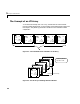

Table Of Contents
- Introduction
- LTI Models
- Operations on LTI Models
- Model Analysis Tools
- Arrays of LTI Models
- Customization
- Setting Toolbox Preferences
- Setting Tool Preferences
- Customizing Response Plot Properties
- Design Case Studies
- Reliable Computations
- GUI Reference
- SISO Design Tool Reference
- Menu Bar
- File
- Import
- Export
- Toolbox Preferences
- Print to Figure
- Close
- Edit
- Undo and Redo
- Root Locus and Bode Diagrams
- SISO Tool Preferences
- View
- Root Locus and Bode Diagrams
- System Data
- Closed Loop Poles
- Design History
- Tools
- Loop Responses
- Continuous/Discrete Conversions
- Draw a Simulink Diagram
- Compensator
- Format
- Edit
- Store
- Retrieve
- Clear
- Window
- Help
- Tool Bar
- Current Compensator
- Feedback Structure
- Root Locus Right-Click Menus
- Bode Diagram Right-Click Menus
- Status Panel
- Menu Bar
- LTI Viewer Reference
- Right-Click Menus for Response Plots
- Function Reference
- Functions by Category
- acker
- allmargin
- append
- augstate
- balreal
- bode
- bodemag
- c2d
- canon
- care
- chgunits
- connect
- covar
- ctrb
- ctrbf
- d2c
- d2d
- damp
- dare
- dcgain
- delay2z
- dlqr
- dlyap
- drss
- dsort
- dss
- dssdata
- esort
- estim
- evalfr
- feedback
- filt
- frd
- frdata
- freqresp
- gensig
- get
- gram
- hasdelay
- impulse
- initial
- interp
- inv
- isct, isdt
- isempty
- isproper
- issiso
- kalman
- kalmd
- lft
- lqgreg
- lqr
- lqrd
- lqry
- lsim
- ltimodels
- ltiprops
- ltiview
- lyap
- margin
- minreal
- modred
- ndims
- ngrid
- nichols
- norm
- nyquist
- obsv
- obsvf
- ord2
- pade
- parallel
- place
- pole
- pzmap
- reg
- reshape
- rlocus
- rss
- series
- set
- sgrid
- sigma
- sisotool
- size
- sminreal
- ss
- ss2ss
- ssbal
- ssdata
- stack
- step
- tf
- tfdata
- totaldelay
- zero
- zgrid
- zpk
- zpkdata
- Index

5 Arrays of LTI Models
5-2
Introduction
In many applications, it is useful to consider collections of linear, time
invariant (LTI) models. For example, you may want to consider a model with a
single parameter that varies, such as
sys1 = tf(1, [1 1 1]);
sys2 = tf(1, [1 1 2]);
sys3 = tf(1, [1 1 3]);
and so on. A convenient way to store and analyze a collection like this is to use
LTI arrays. Continuing this example, you can create this LTI array and store
all three transfer functions in one variable.
sys_ltia = (sys1, sys2, sys3);
YoucanusetheLTIarraysys_ltia just like you would use, for example, sys1.
You can use LTI arrays to collect a set of LTI models into a single MATLAB
variable. You then use this variable to manipulate or analyze the entire
collection of models in a vectorized fashion. You access the individual models
in the collection through indexing rather than by individual model names.
LTI arrays extend the concept of single LTI models in a similar way to how
multidimensional arrays extend two-dimensional matrices in MATLAB (see
Chapter 12, “Multidimensional Arrays” in Using MATLAB).
When to Collect a Set of Models in an LTI Array
You can use LTI arrays to represent:
•A set of LTI models arising from the linearization of a nonlinear system at
several operating points
•A collection of transfer functions that depend on one or more parameters
•A set of LTI models arising from several system identification experiments
applied to one plant
•A set of gain-scheduled LTI controllers
•A list of LTI models you want to collect together under the same name
Restrictions for LTI Models Collected in an Array
For each model in an LTI array, the following properties must be the same: