TI-83, TI-83 Plus and the TI-84 GRAPHING CALCULATOR MANUAL James A. Condor Manatee Community College to accompany Introductory Statistics Sixth Edition by Prem S. Mann Eastern Connecticut State University JOHN WILEY & SONS, INC.
Contents Preface 3 1 Introduction 4 2 Organizing Data 11 3 Numerical Descriptive Measures 17 4 Probability 27 5 Discrete Random Variables 32 6 Continuous Random Variables 39 7 Sampling Distributions 46 8 Estimation of the Mean and Proportion 50 9 Hypothesis Tests: Mean and Proportion 55 10 Two Populations 61 11 Chi-Square Tests 69 12 Analysis of Variance 74 13 Simple Linear Regression 78 14 Nonparametric Methods 84 2
Preface Statistics is an important field of study, now more so than ever. We are surrounded by statistical information in work and in our everyday lives. Many of us work in professions that require us to understand statistical summaries, and some of us work in areas that require us to produce statistical information. The art of teaching statistics has changed dramatically in recent years, with computational software eliminating the need for many of the previously taught techniques.
Chapter 1 Introduction Use of Technology Statistics is a field that deals with sets of data. After the data is collected it needs to be organized and interpreted. There is a limit to how much of the work can be done effectively without the help of some type of technology. The use of technology, such as a calculator with enhanced statistical functions can take care of most of the details of our work so that we can spend more time focusing on what we are doing and how to interpret the results.
Advantages to Using the TI-83, TI-83 Plus, and TI-84 Plus This calculator manual will focus on how to get the most out of using the TI-83, TI-83 Plus, and the TI-84 Plus calculators by Texas Instruments. The TI-83 was first released in 1996, improving upon its predecessors the TI-81 and TI-82 with the addition of many advanced statistical and financial functions.
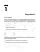
Press the STAT key. To input data or to make changes to an existing set of data values use the Edit function. (number one under the EDIT list). Press the number 1 key. If your stat list editor does not show the columns labeled L1, L2, and L3 you can set up the Editor by selecting SetUpEditor on the previous screen. Press the STAT key. Press the 5 key. Press the ENTER key. If you set up the editor then return to the Edit function. Go ahead and type the ten weights in under the column labeled L1.
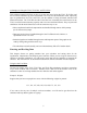
Use the up and down arrow keys to go back and forth between the numbers. Try changing the value of one of the entries by typing in a new weight. Clearing a List of Data Values After a list of data values is no longer needed you can delete the values by using one of the following methods. 1. You can highlight each data value and use the DEL key. This method is slow and clears the list one data value at a time. 2.
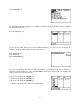
You can also store data to a name that you create. From the home screen, you can save a list to a name by using the STO► key. {131, 114, 167, 180, 126, 134, 188, 175, 133, 130} → WEIGH If you type in WEIGH on the home screen and press the ENTER key the list of numbers will be displayed across the screen. Next we will learn how to create a different name for a list rather than using L1, L2, and so on.
LIST menu, and choose one of the list names there by using the arrow keys and then press the ENTER key. In general, when you need to supply the name of a list to a command or a menu, use the LIST page and the NAMES list. Choosing Lists to Edit There are several ways to control which lists are displayed in the Stat List Editor. If you press the STAT key and then the number 5 key to get to SetUpEditor, you can use that command with a series of list names separated by columns.
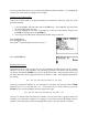
Exercises 1. Store the following numbers into the list L2: 11, 23, 35, 47, 59 2. Store the following numbers into the list ABC: 2, 3, 5, 7, 11, 13 3. Configure the Stat List Editor to display lists L2, ABC, and L5. 4. Save the following data in a storage location labeled TIME. 23, 45, 56, 32, 42, 22 Solutions 1. Go to the STAT page and select Edit. If L2 is not one of the lists displayed, use the up arrow to highlight one of the column titles, press INS for insert and press the ENTER key.
Chapter 2 Organizing Data After the data has been input into the calculator one of the tasks of the statistician is to try to make sense of that data by organizing it. As a consumer of statistics, you are presented with tables and graphical displays of data on a daily basis. This chapter focuses on ways of organizing data on the TI-83, TI-83 Plus, and TI-84 Plus calculators. Frequency Distributions One of the simplest ways of organizing data is to group together similar values.
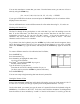
Team Home Runs Team Home Runs Anaheim Arizona Atlanta Baltimore Boston Chicago Cubs Chicago White Sox Cincinnati Cleveland Colorado Detroit Florida Houston Kansas City Los Angeles 152 165 164 165 177 200 217 169 192 152 124 146 167 140 155 Milwaukee Minnesota Montreal New York Mets New York Yankees Oakland Philadelphia Pittsburgh St. Louis San Diego San Francisco Seattle Tampa Bay Texas Toronto 139 167 162 160 223 205 165 142 175 136 198 152 133 230 187 Press the WINDOW key.
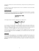
Press the GRAPH key. Press the TRACE key. Use the arrow keys to move from one bar to the other. (this will supply information on the frequency in each category and the range of values in each category). The histogram provides us with the following information. _Class_ 124-145 146-167 168-189 190-212 213-234 Frequency 6 13 4 4 3 Lets review the steps for creating a histogram. 1. Enter the data into a list. 2. Determine the range of values for your data, as well as your desired class width. 3.
We’re going to construct a frequency histogram from the data. The data ranges from 15.4 to 31.2 so we will have our classes go from 15 to 33. That is a range of 33 − 15 = 18, so we will construct six classes of width 3. Go into the Stat List Editor and create a new list called WORK. Enter the times. Press the STAT key. Press the number 1 key. Press the 2nd key and then the DEL key to get to INS. Type in WORK and then press the ENTER key. Enter the data values.
Creating a Dotplot You can create a Dotplot by using the scatterplot option under STATPLOT. The steps to create the dotplot are very similar to those needed to create the histogram. We will use the data stored under the label WORK that we used to create the histogram in the previous example. Press the STAT key. Press the number 1 key. Type in the numbers 1 through 50 in the L1 column. Press the 2nd key and then the Y= key to get to STATPLOT. Press the number 1 key.
Exercises 1. Take the following statistics exam scores and construct a frequency histogram for them with classes from 50 to 59, from 60 to 69, from 70 to 79, from 80 to 89, and from 90 to 99. 95 95 54 82 80 63 90 57 76 71 90 95 87 96 69 73 67 84 92 55 83 73 68 72 77 57 93 55 54 98 93 71 78 92 85 84 69 76 96 81 2. Create a dot plot using the above data values. Solutions 1. Enter the data into a list. In STAT PLOT turn one of the plots on, and choose a frequency histogram as the type.
Chapter 3 Numerical Descriptive Measures After data is collected and organized the next step is usually to generate descriptive statistics. Descriptive statistics helps you describe the contents of the data set. The two most common measures are measures of central tendency and measures of variability. These measures tell you where the data is centered and how spread out it is.
Example: Prices of CDs. The following data values are the prices of the same popular CD sold from ten different discount stores. 12.95, 14.90, 11.57, 14.65, 17.95, 21.25, 12.95, 20.35, 10.95, 25.05 Press the STAT key. Press the number 1 key. Enter the data values into L1. Press the STAT key. Press the ► key to highlight CALC. Press the number 1 key to select 1-Var Stats. Press the 2nd key and then the number 1 key to get L1. Press the ENTER key.
The last five numbers (minimum, first quartile, median, third quartile, and maximum) are collectively known as the five-number summary of the data. From the five-number-summary we can compute the range, which is the difference between maxX and minX, and the interquartile range, which is the difference between Q3 and Q1. Example: Average Payroll The following list of data values lists the 2002 total payroll for five Major League Baseball teams. Let’s analyze the five payrolls.
The first line displays the sample mean, Ë = 78 million dollars. The fourth line displays the sample standard deviation, Sx = 34.4 million dollars. Use the down arrow key to see that the median payroll is 75 million dollars. The interquartile range is found by subtracting the two quartiles Q3−Q1 = 109.5 − 48 = 61.5 million dollars. The range is maxX − minX = 126 − 34 = 92 million dollars. Example: Concert Revenues The following table contains the top twelve concert revenues of all time.
Grouped Data Sometimes a set of data values has many numbers that show up over and over again. Instead of typing those numbers in over and over again you can save time by typing in the numbers that repeat along with how many times it repeats. Example: Multiple Frequencies The following is a list of data values that are ungrouped.
Press the STAT key. Press the number 1 key. Enter the times in L1. Enter the frequencies in L2. Press the STAT key. Press the ► key to Highlight CALC. Press the ENTER key. Type in L1, L2. Press the ENTER key. The sample mean and median are 9.22 and 8 minutes, respectively. The sample standard deviation is 3.1 minutes, the range is 12 minutes, and the interquartile range is 2.5 minutes.
Elementary Statistics Final Exam Scores 76 81 56 76 88 90 71 60 94 62 77 84 73 94 85 73 Enter the exam scores into a list with the name FINAL. Press the STAT key. Press the number 1 key. Press the ▲ key to highlight L1. Press the 2nd key and then the DEL key to get to INS. Type in FINAL for the name of the new list. Type in the exam scores. Press the STAT key. Press the number 3 key to get the function SortD( . Press the 2nd key and then the STAT key to get to LIST.
Box-and-Whisker Plot The TI-83, TI-83 Plus, and TI-84 Plus calculators will take a list of data and automatically draw a box-and-whisker plot for that data. Since there are a number of different types of plots available on the calculator, it is important to make sure that all other plots are turned off before you begin or you graph will be cluttered with several unrelated plots being graphed at the same time.
Set the Freq: to 1. Press the ZOOM key. Press the number 9 key. We have two different types of box-and-whisker plots to select from. One will separate outliers from the maximum or minimum value and the other will include the outliers in to whiskers. If you select the picture that shows two dots after the maximum on the plot, the outliers will be shown outside of the whiskers.
Exercises 1. Find the mean and sample standard deviation for the following data: 34 23 55 91 23 34 12 34 98 23 2. Find the median and interquartile range for the following grouped data: Score 34 27 84 72 86 59 22 Frequency 9 11 4 14 8 12 9 3. What is the percentile rank of 82 in the following data? 68 89 77 71 57 90 97 82 58 69 89 38 39 4. Create a box-and-whisker plot for the following data: 71 23 19 34 42 21 5 11 32 Solutions 1. The sample mean Ë = 42.7.
Chapter 4 Probability Generating Random Numbers When working with probabilities, it is sometimes useful to generate numbers that you can’t predict, but at the same time follow some standard rules. Computer simulations are a common example of the need for random occurrences within a structured setting. These numbers are called pseudo-random numbers since they are not totally random. Your calculator can generate these types of random numbers.
Press the ENTER key. Press the ENTER key again. If you continue to press the ENTER key you will generate a different random number between zero and one each time you press the ENTER key. Generating Random Numbers Between any Two Values If you would like to generate random real numbers that are equally likely to occur and fall within a specified range of values you can use the rand function with some additional commands.
After the randInt( function appears on your screen you can type in the minimum and maximum values for the range of random numbers you are searching for. The minimum value goes first followed by a comma and then the maximum value. For this example we are looking for random integer values between 1 and 100 so your finished typing would be randInt(1,100). Each time you press the ENTER key a different random integer will appear. In general the syntax would look like randInt(minimum, maximum).
The syntax for these functions are similar to those needed for the randInt( function. For example, if you wanted to generate 30 numbers from a normal distribution with a mean of 45 and a standard deviation of 8 and store them in L2 you would select number 6 and type in randNorm(45, 8, 30)→L2. The general syntax needed is randNorm(µ, σ, number). The syntax for the randBin( to generate random numbers from a binomial distribution is randBin(n, p).
Exercises 1. Create a random integer value between 50 and 60 inclusive. 2. Create a random real number between 3 and 17. 3. Generate 15 random integer values between 1 and 50 and store them in L1. 4. Select 10 values from a normally distributed population with a mean of 22 and a standard deviation or 2.6. Solutions 1. Type randInt(50, 60). 2. Type rand*(17-3)+3. 3. Type randInt(1, 50, 15)→L1. 4. Type randNorm(22, 2.
Chapter 5 Discrete Random Variables and Their Probability Distributions Mean and Standard Deviation of a Discrete Random Variable Computing the mean and standard deviation of a discrete random variable is slightly different than computing the mean and standard deviation of a set of data values. Each data value in the data set weighs equally in the computation. In a discrete random variable the possible data values are given along with the likelihood of each value occurring on any given single trial.
Press the STAT key. Press the number 1 key. Enter the x values into L1. Enter the P(x) probabilities into L2. Press the STAT key. Press the ► key to highlight CALC. Press the number 1 key When 1-Var Stats appears on the calculator screen, type in L1, L2 to get 1-Var Stats L1, L2. After you press the ENTER key you will get the descriptive statistics which includes the population mean and standard deviation.
Permutations Another common function needed to compute dependent probabilities that uses factorial is the permutation formula. The number of permutations is normally written as nPr; on the calculator with the symbol P written between n and r, where n is the total number of elements, and r is the number being selected. Permutations are used when trying to find all possible arrangements of elements taken from a larger selection.
Binomial Probabilities The command for computing binomial probabilities is binompdf( , which is located on the DISTR page (which is found in yellow above the fourth key in the fourth row). To find the probability of x successes out of n trials, each with probability p of success, type binompdf(n, p, x). Example: VCR’s Suppose that 5% of all VCR’s manufactured by an electronics company are defective. Three VCR’s are selected at random.
Find the probability that at most 2 or less of these 10 packages will not arrive at its destination within the specified time. Press the 2nd key and then press the VARS key to get to the DISTR page. Press the ALPHA key and then press the MATH key to get to the letter A which is the binomcdf( function. After binomcdf( appears on the screen, type in 10, .07, 2). Press the ENTER key. The result is 0.9716578543 or ≈ 97.2%.
Example: New Bank Accounts Suppose that on the average two new accounts per day are opened at an Imperial Savings Branch bank. Let’s find the probability that on a given day at least 7 new accounts are opened. The complement of opening at least 7 new accounts is opening at most 6 new accounts, which has probability poissoncdf(2, 6) = 0.9955. The probability of opening at least 7 new accounts is 1−0.9955 = 0.0045.
Exercises 1. Find 13! 2. Find the number of ways to deal a five-card hand from a deck of 52 cards. 3. Find the number of four-digit numbers that don’t have any digits repeated. 4. A company has 50 fork-lifts. On any given day each fork-lift has a 1% chance of needing maintenance. What is the probability that today 3 forklifts will need maintenance? 5. For the same company, what is the probability that at most 5 trucks will need maintenance today? 6. A small store has on the average 23 customers per day.
Chapter 6 Continuous Random Variables and the Normal Distribution Continuous random variables are used to approximate probabilities where there are many possibilities or an infinite number of possibilities on a given trial. One of the most common continuous distributions used to approximate probabilities is the normal distribution. Traditionally normal distribution probabilities were figured using a normal distribution table.
Press the 2nd key and then the VARS key to get to the DISTR page. Press the number 1 key. Type in 1, 0, 1) to get normalpdf(1,0,1). Press the ENTER to get .242. To find the probability of getting a value that falls within a range of values from the standard normal distribution you can use the normalcdf( function which stands for normal cumulative density function.
Press the number 2 key. Type in the number -1. Press the 2nd key and then the , (comma) key to get the exponential sign E. Type in 99, 0, 1) after the E. Press the ENTER key. The probability is .159. Example: Finding the Area to the Right To find the area to the right of a number a, type normalcdf(a, 1E99). The E is for scientific notation, and is located above the comma key in the sixth row (where the label appears as EE).
Example: Finding the Area Between two values. To find the area between two numbers a and b, type normalcdf(a, b, 0, 1). Find the probability of getting a value between 1.04 and 1.82 on the standard normal distribution. Press the 2nd key and then the VARS key to get to the DISTR page. Press the number 2 key. Type in the number 1.04, a comma, and then 1.82. Type the mean and standard deviation 0, 1 and then ). Press the ENTER key. The probability is .115.
Find the probability of getting a score less than 32 given the distribution is normally distributed with a mean of 45 and a standard deviation of 12. Using the normalcdf( function and typing in -1E99, then the score 32 with a mean of 45 and standard deviation of 12 we get the probability .139. Example: Soda Cans Suppose that the contents (in ounces) of a soda can labeled “12 ounces” follows a normal distribution, with mean 12 and standard deviation 0.015.
To find the score that is associated with the lowest 1% of the area under the normal distribution we use invNorm( . Press the 2nd key and then the VARS key to get to the DISTR page. Press the number 3 key. Type in .01, 54, 8). Press the ENTER key. We should offer to replace defective calculators up to 35 months old. Example: SAT Scores Given that the 2002 SAT scores were normally distributed with mean 1020 and standard deviation 153, what is the 90th percentile score? invNorm(0.90, 1020, 153) = 1216.
Exercises 1. What is the probability that a z-score will lie between 2 and 3? 2. How likely is it for a z-score to be over 2.5? 3. What is the chance that a z-score is less than 1.3? 4. The heights in inches at a certain age are normally distributed with mean 48 and standard deviation 3.2. What is the probability that a person at that age is over 53 inches tall? 5. The pH (a measurement of acidity) in a lake is normally distributed with mean 6.8 and standard deviation 0.43.
Chapter 7 Sampling Distributions A large part of statistics consists of analyzing the probability of getting a sample mean or sample proportion from a repeated number of samples drawn from the same population. Usually we focus on two kinds of statistics from those samples: the sample mean Ë, if the data is quantitative, or the sample proportion ê, if the data is categorical. For large sample sizes, both Ë and ê have normal distributions which makes it much easier to compute their associated probabilities.
Press the 2nd key and then press the VARS key to get to the DISTR page. Press the number 2 key. Type in -1E99, 31.8, 32, .3/ 20 )) Press the ENTER key. The probability is .0014. Example: Tuition According to a recent College report, the average tuition and fees at four year private colleges and universities in the United States is $18,273 for the academic year 2002–2003. Suppose that the tuition’s exact distribution is unknown but its mean is $18,273 and its standard deviation is $2100.
Probabilities for Sample Proportions For a large sample size, we know from the Central Limit Theorem that the sampling distribution for ê is normally distributed with µê = p and σê = pq / n To find the probability that a < ê < b on the calculator, use normalcdf(a, b, p, pq / n ). Note that it is more accurate to type pq / n directly into the normalcdf( command than to compute it separately and type it in.
Exercises 1. Assume that the average annual family income in a given city is $28,000 with standard deviation $3200. If a random sample of fifty families is taken, what is the chance that the average income of the fifty families will be over $29,000? 2. Assume that 2% of all light bulbs produced at a factory are defective. If a random sample of 150 bulbs is taken, what is the probability that less than 4% of the sample bulbs are defective? Solutions 1. normalcdf(29000, 1E99, 28000, 3200/ 50 ) = .013 = 1.3%.
Chapter 8 Estimation of the Mean and Proportion In statistics we collect samples to find things out about a population. If the sample is representative of the population, the sample mean or proportion should be statistically close to the actual population mean or proportion. A way to judge how close the sample statistic may be is to create a confidence interval. This chapter will describe how to use the calculator to compute confidence intervals for population means and proportions.
Press the STAT key. Press the ► twice to highlight TESTS. Press the number 7 key. The first line under ZInterval has two options for Inpt: Data Stats. If the mean and standard deviation are given in the problem then Stats should be selected. If the data values are given in the problem then Data should be selected. In this problem the mean and standard are given. Select Stats by moving the cursor over Stats and then press the ENTER key. Type in 4.5 for σ. Type in 70.5 for Ë. Type in 36 for n. Type in .
We do not have the population standard deviation σ, so we will use TInterval. Press the STAT key. Press the ► key twice to highlight TESTS. Press the number 8 key. We do not have the data itself, so we will select Stats. We enter 15,528 for Ë, 4200 for sx, 400 for n, and .99 for the C-Level. Select Stats for Inpt: and press the ENTER key. Type in 15528 for Ë. Type in 4200 for Sx. Type in 400 for n. Type in .99 for C-Level. Highlight Calculate and press the ENTER key.
Example: Legal Advice According to a 2002 survey by FundLaw, 20% of Americans needed legal advice during the past year to resolve such thorny issues as trusts and landlord disputes. Suppose a recent sample of 1000 adult Americans showed that 20% of them needed legal advice in the past year to resolve such family-related issues. Find a 99% confidence interval for the percentage of American adults who needed such legal advice.
Exercises 1. Given that σ = 4 for a given population and the following sample data, find a 95% confidence interval for µ. 24 31 31 34 18 22 2. Find a 90% confidence interval for µ given the following sample data from a normal population: 87 97 67 88 97 73 81 3. In a random sample of 350 town residents, 230 of them have cable television. Find a 95% confidence interval for the percentage of all town residents who have cable television. 4.
Chapter 9 Hypothesis Tests About the Mean and Proportion Hypothesis Tests About Means Hypothesis tests about means can be Z-based (if σ is known) or T-based (if σ is unknown and either the population is normal or the sample size is over 30). The TI-83, TI-83 Plus, and the TI84 Plus calculators provide functions for both the Z-Test and the T-Test. They both provide a pvalue for comparison with the test’s significance level.
Press the STAT key. Press the ► key twice to highlight TESTS. Press the number 2 key. Move the cursor over Stats and press the ENTER key. Type in 50352 for µ0. Type in 51750 for Ë. Type in 5240 for Sx. Type in 200 for n. Move the cursor over >µ0 and press the ENTER key. Move the cursor over Calculate and press the ENTER key. The T-Test output shows the alternative hypothesis: µ>50352 test statistic: t=3.77303543 p-value: 1.
Press the STAT key. Press the ► key twice to highlight TESTS. Press the number 2 key. Move the cursor over Stats and press the ENTER key. Type in 65 for µ0. Type in 63 for Ë. Type in 2 for Sx. Type in 15 for n. Move the cursor over <µ0 and press the ENTER key. Move the cursor over Calculate and press the ENTER key. The T-Test output shows the alternative hypothesis: µ<65 test statistic: t=-3.872983346 p-value: p=8.
defective chips. Test at the 5% significance level whether or not the machine needs an adjustment. Our hypotheses are H0: p = 4% and H1: p > 4%. We will use 1-PropZTest, with p0 = 0.04, x = 14, n = 200, and p1 > p0 for our alternative hypothesis. Press the STAT key. Press the ► key twice to highlight TESTS. Press the number 5 key. Type in .04 for p0. Type in 14 for x. Type in 200 for n. Move the cursor over >P0 and press the ENTER key. Move the cursor over Calculate and press the ENTER key.
Press the STAT key. Press the ► key twice to highlight TESTS. Press the number 5 key. Type in .9 for p0. Type in 129 for x. Type in 150 for n. Move the cursor over
Exercises 1. Test at a 5% significance level whether or not µ = 98 given the following sample data from a normal population: 97 105 90 89 112 130 2. Test at a 5% significance level whether or not p is more than 75%, given a sample proportion of 80% and a sample size of 235. Solutions 1. We are testing Ho : µ = 98 versus H1 : µ ø 98. Enter the data into a list, then use T-Test with Data selected. Using µ0 = 98 and µøµ0 as the alternative hypothesis, we find that the p-value is 0.401.
Chapter 10 Estimation and Hypothesis Testing: Two Populations Confidence Interval for µ1 − µ2 If you are fortunate enough to have information about the population standard deviations, you can use 2-SampZInt to estimate the difference µ1 − µ2 between two population means. The most general approach, though, to estimating the difference of two population means is to compute a T-based confidence interval, which does not make any assumptions about the population’s standard deviations.
Press the STAT key. Press the ► key twice to highlight TESTS. Press the number 9 key. Move the cursor over Stats and press the ENTER key. Type in 9000 for σ1. Type in 8500 for σ2. Type in 49056 for Ë1. Type in 500 for n1. Type in 46800 for Ë2. Type in 400 for n2. Type in .95 for the C-Level. Move the cursor over Calculate and press the ENTER key. The 2-SampZInt output shows the: confidence interval: (1108.8, 3403.2) sample means and sample sizes. The 95% confidence interval for µ1 − µ2 is ($1108.8, $3403.
Example: Average Salaries Test at the 1% significance level if the 2001 mean salaries of full-time state employees in New York and Massachusetts are different. We are testing to choose between H0: µ1 = µ2 and H1: µ1 ø µ2. Since we have the population standard deviations, we will use 2-SampZTest. Press the STAT key. Press the ► key twice to highlight TESTS. Press the number 3 key. Move the cursor over Stats and press the ENTER key. Type in 9000 for σ1. Type in 8500 for σ2. Type in 49056 for Ë1.
Pretest/Posttest. Data is collected from a sample before some type of treatment and then data is collected again from that same sample after the treatment. We then work with the mean difference between the pre and posttest scores. The null hypothesis is that the average difference is zero. By working with the differences between the variables, we can perform a one-sample TTest. Example: Blood Pressure A researcher wanted to find the effects of a special diet on systolic blood pressure.
The T-Test output shows the: alternative hypothesis: µ>0 test statistic: t=1.226498265 p-value: p=.1329778401 sample mean: Ë=5 sample standard deviation: Sx=10.78579312 sample size: n=7 The p-value is greater than the significance level so we accept the null hypothesis of no significant difference between the pre and posttest scores. There is not enough evidence to claim that the special dietary plan was effective in lowering systolic blood pressure.
Enter in the data for the 2-PropZTest. Highlight Calculate and press the ENTER key. The test statistics is 1.15 and the p-value is .13. Since the p-value is larger than the significance level of 1% we accept the null hypothesis. There is not enough evidence to claim significant differences between toothpaste loyalties.
Exercises 1. Given the following sample data from two populations, find a 95% confidence interval for µ1 − µ2: Ë1 = 23.5 s1 = 5.1 n1 = 38 Ë2 = 17.9 s2 = 2.4 n2 = 59 2. Given the following paired data, test at a 5% significance level whether or not µ1 = µ2. x 13 32 12 14 35 y 43 92 74 77 71 3. Given the following sample data, test at a 5% significance level whether or not p1 < p2. ê1 = 23% n1 = 89 ê2 = 37% n2 = 143 4.
Solutions 1. Since we do not have the population standard deviations, we will use a T-based confidence interval, 2-SampTInt, and select Stats. We enter the sample statistics and choose No for the Pooled prompt since we do not know that the population standard deviations are equal. The confidence interval is (3.82, 7.38). 2. This is paired data, so we need to examine the differences of the values. We enter the two sets of measurements into L1 and L2, and take their difference as L3.
Chapter 11 Chi-Square Tests Contingency Tables When you are measuring the relationship between two categorical variables, one of the most important tools for analyzing the results is a two-way frequency table. We can use the table to see if the variables are independent by comparing observed frequencies with the frequencies that would be expected from such a sample if they were independent. A Chi-Square (Χ2) test-statistic can be computed from the observed and expected frequencies.
Test at a 5% significance level whether or not Gender and Opinion are independent. Then check the expected frequencies for any possible practical significant differences between the associated observed and expected frequencies. First the data has to be stored differently than in previous statistical test on the calculator. The data for a Chi-Square test of independence has to be stored in a Matrix. Press the 2nd key and then the x-1 key to get to MATRX. Press the ► key twice to highlight EDIT.
Since the p-value of .016 is less than the significance level of .05 we reject the null hypothesis that row and column variables are independent. We have evidence that gender does influence opinions concerning school discipline. The see the expected frequencies Press the 2nd key and then the x-1 key. Press the ► key twice to get to EDIT. Press the number 2 key to get to [B]. Comparisons such as 70 men were against giving more freedom to teachaers to punish kids and we only expected 59.
After MATRIX [A] type in 2 x2. The 2 represents the number of rows in the table. The 2 represents the number of columns in the table. Press the ENTER key. Enter the data values into the matrix as they appear in the table. Press the STAT key. Press the ► key twice to get to TESTS. Press the ALPHA key and then the PRGM key to get to C: X2-Test… The X2-Test output shows: That the observed values are in matrix A That the expected values are in matrix B Move the cursor to Calculate and press the ENTER key.
Exercises 1. Test at a 5% significance level whether or not state and blood type are independent of each other using the following sample data. New York California Type O 50 125 Type A 40 100 Type B 35 120 Type AB 10 30 2. Test at a 5% significance level whether or not car ownership and cell phone ownership are independent of each other using the following sample data. Owns Car Does Not Own Car Owns Cell Phone 500 125 Do Not Own Cell Phone 140 80 Solutions 1. The p-value is .58.
Chapter 12 Analysis of Variance One-Way Analysis of Variance We have already seen how to test for the equality of means between two different populations with 2-SampZTest and 2-SampTTest. With the added assumption of common population standard deviations, we can extend the tests to more than two populations with a technique known as Analysis of Variance (ANOVA for short). The null hypothesis is that all of the population means are equal; the alternative hypothesis is that at least two of the means differ.
Press the STAT key. Press the ENTER key to get to the Stat Editor. Enter the Method I data values into L1. Enter the Method II data values into L2. Enter the Method III data values into L3. Press the STAT key. Press the ► key twice to highlight TESTS. Press the ALPHA key and then the COS key to get to ANOVA. Type in L1, L2, L3). Press the ENTER key. The One-way ANOVA output shows the: test statistic: F = 1.092717465 p-value: P=.
Teller A 19 21 26 24 18 Teller B 14 16 14 13 17 13 Teller C 11 14 21 13 16 18 Teller D 24 19 21 26 20 At a 5% level of significance, test the null hypothesis that the mean number of customers served per hour by each of the four tellers is the same. Assume all the assumptions required to apply the one-way ANOVA procedure hold true. Press the STAT key. Press the ENTER key. Enter the Teller A scores into L1. Enter the Teller B scores into L2. Enter the Teller C scores into L3.
Exercises 1. Test at a 5% significance level whether or not these samples come from populations with identical means. Assume that the populations are all normally distributed with identical standard deviations. A 10 13 18 16 19 B 15 17 15 14 18 14 C 12 15 13 14 17 19 D 16 10 13 18 12 Solutions 1. The p-value is .779. Accept the null hypothesis. The population means are not significantly different from each other.
Chapter 13 Simple Linear Regression Simple Linear Regression Models A simple linear regression model is an equation describing how to use one variable x to predict another y, based on the relationship that we see in sample data. Since we are making predictions that may differ from the actual values, we use the symbol y' for the predicted value of y. The simplest possible model is a linear one: y' = a + bx.
Press the STAT key. Press the number 1 key. Type the English scores in L1 Type the Math scores in L2. Press the 2nd key and then the Y= key to get to STATPLOT. Press the number 1 key. Turn Plot1 On and highlight the scatterplot under Type. Type L1 in for the Xlist: Type L2 for the Ylist: Select any one of the symbols Mark: Press the Zoom Key. Press the number 9 key to get to ZoomStat. If you would like to see the coordinates of the marks, press the TRACE key.
Press the STAT key. Press the ► key. Press the number 8 key. Press the 2nd key and then the number 1 key to get L1. Press the , (comma) key. Press the 2nd key and then the number 2 key to get L2. Press the , (comma) key. Press the VARS key. Press the ► key. Press the ENTER key. Press the number 1 key to get Y1. Press the ENTER key. The LinReg output shows the: general model: y=a+bx y-intercept: a=79.1116729 slope: b=-.053528248 coefficient of determination: r2=.
Hypothesis Tests Just because we can compute a regression model does not mean that it is a valid model. We can test whether or not the variable x can meaningfully predict the variable y by running LinRegTTest to test whether or not B, the population slope coefficient for the model (approximated by b) is really 0. LinRegTTest is located on the STAT page in the TESTS list. The test requires the names of the lists containing the data values and what the alternative hypothesis is.
Type in L1, L2, Y1. Press the ENTER key. The LinReg output shows the: general model: y=a+bx y-intercept: a=1.142245989 slope: b=.264171123 coefficient of determination: r2=.9190178504 linear correlation coefficient: r=.9586541871 We perform the test of H0: B = 0 versus H1: B > 0 in LinRegTTest. Press the STAT key. Press the ► key twice to highlight TESTS.
Exercises Use the following sample data for the exercises in this chapter. Height (in) Weight (lbs) 67 195 71 220 62 100 66 168 74 225 64 130 72 180 74 190 1. Compute a regression model for this data and also find the coefficient of determination and the linear correlation coefficient. 2. Use the model to estimate the weight of someone who is 5’8”, i.e., 68 inches tall. 3. Sketch a scatter diagram with the regression line. 4.
Chapter 14 Nonparametric Methods Sign Test The Sign Test is one of the most direct nonparametric methods; knowing nothing about the distribution, we can still test claims about the median of a population because any sample measurement stands a 50% chance of being above the median and a 50% chance of being below the median. We can treat sample data as being a binomial experiment, with successes occurring when the measurement is above the median.
Home Price 1 147,500 2 123,600 3 139,000 4 168,200 5 129,450 6 132,400 7 156,400 8 188,210 9 198,425 10 215,300 Using a 5% significance level, can we conclude that the median price differs from $137,000? Our hypotheses are H0 : the median price is $137,000 versus H1 : the median price differs from $137,000. We replace the sample prices by signs: + if the price is above the hypothetical median $137,000, and − if it is below. Home Price 1+ 2−3+ 4+ 5−6−7+ 8+ 9+ 10 + We have seven +’s out of ten signs.
Our hypotheses are H0 : the median is at least $70 versus H1 : the median is less than $70. For a large sample size (n = 89 households that were above or below $70) we can use 1-PropZTest. The p-value is 0.084, which is greater than our significance level. We fail to reject the null hypothesis, and believe that the median price is at least $70. Medians of Paired Data Given paired data, we can test to see if the medians of their respective populations are the same by applying a signs test.
Since the p-value is less than our significance level 2.5%, we reject the null hypothesis. The data leads us to conclude that the diet does lower the median systolic blood pressure of adults. Example: Math Anxiety Many students suffer from math anxiety. A statistics professor offered her students a two-hour lecture on math anxiety and ways to overcome it. A total 79 of 42 students attended this lecture. The students were given similar statistics tests before and after the lecture.
Index 1-Var Stats, 13 analysis of variance, 65 ANOVA, 65 binomial distribution, 28 binomial probabilities, 28 box-and-whisker plot, 20 Central Limit Theorem, 39 combinations, 28 confidence interval, 43 confidence interval for µ, 43 confidence interval for p, 47 contingency tables, 59 creating lists, 4 cumulative binomial probability, 29 data entry, 2 data, entering, 2 data, grouped, 13, 17, 18 data, revising, 2 data, ungrouped, 13 distribution, binomial, 28 distribution, geometric, 31 distribution, inverse
minimum, 14 naming lists, 4 nonparametric methods, 75 normal distribution, 34 normal probabilities, 34 numbers, pseudo-random, 23 numbers, random, 23 observed frequencies, 59 percentiles, 19 plot, box-and-whisker, 20 Poisson distribution, 30 Poisson probabilities, 30 population standard deviation, 14 probabilities, sample mean, 39 probabilities, sample proportion, 40 pseudo-random numbers, 23 quartile, first, 14 quartile, third, 14 random numbers, 23 range, 15 range, interquartile, 15 revising data, 2 sampl