
Intel Xeon Processor Multiprocessor Platform Design Guide

104
Methodology for Determining Topology and Routing Guidelines
9.2.6.1 Parameter Sweeps
The bulk of the sensitivity analysis consists of parameter sweeps. During a parameter sweep all
parameters are held constant except for one or two. The system performance is then observed as the
specific variables are being swept. Surface plots can be generated from the results of the parameter
sweep. Then the timing and signal quality specifications can be superimposed onto the surface and
design limits such as line length, buffer strength, line impedance, etc. can be determined.
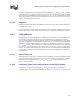
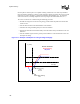
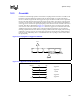
Figure 9-11 shows an example of surface plots based on simulated flight times and undershoot. The
upper and lower left surface plots show flight time as a function of line lengths L2 and L3.
Additional planes are incorporated into the plots that represent the upper and lower flight time
specifications. The upper right plot depicts a signal quality metric as a function of L2 and L3 line
length. The surfaces of all three of these plots are intersected with the specifications and the
resultant solution space for these variables under the conditions of the simulation is shown in the
lower right hand side of Figure 9-11.
It should be noted that the sweeps should be performed using different switching patterns in order
to capture the majority of ISI effects. If N is the fastest switching speed for a given bus, then
simulations should be performed at a frequency of N, ½N, and ¼N. The difference between the
timings at the different switching frequencies is a good approximation of the ISI noise. Final
checks on fully coupled models with long worst-case bit patterns should be performed in order to
find any ISI effects not captured in this analysis. This sweeping technique can be used extensively
to get initial bounds on all variables in the system. The resultant solution space will be known as
the “phase 1 solution space.”
The drawback of this method is that the sweeps are only good for evaluating two variables at a
time. While the two parameters of interest are being varied, the other parameters in the system are
held constant at a value that may not yield worst-case performance. For example, if the line lengths
are being swept all line and buffer impedances, package parasitic effects, receiver capacitance, etc.
are held at fixed values. Every effort should be made to set these parameters so that the
performance will approach worst case. Use Intel's recommendations as a baseline, and work from
there to refine corner conditions specific to your environment. In order to ensure that the worst-
case performance is captured, all system variables must be varied simultaneously. This can be
accomplished using a targeted Monte Carlo analysis.
9.2.6.1.1Targeted Monte Carlo Analysis
Targeted Monte Carlo (TMC) analysis can be used to further refine the phase 1 solution space and
ensure that the worst-case performance has been captured. Performing a full Monte Carlo analysis
over all system variables is inefficient because a large number of simulations must be performed to
statistically guarantee that all worst case conditions are captured. If a TMC analysis is performed
on the boundaries of the phase 1 solution space determined by the parametric sweeps, the number
of simulations required will decrease dramatically and the solution space can be refined by
changing the variables that were held constant during the sweep.
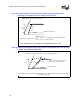
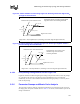
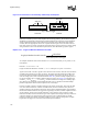
Figure 9-12 shows the area where the TMC analysis was performed to refine the phase 1 solution
space illustrated in Figure 9-11. Figure 9-13 shows the results of the TMC analysis and shows the
final solution space. This final solution space will be referred to as the “phase 2 solution space.” It
should be noted that the worst-case bit pattern should be included in the TMC analysis.