?88,.d88b, d8888b d8888b 88bd8b,d88b .d888b, ‘?88’ ?88d8P’ ?88d8b_,dP 88P’‘?8P’?8b ?8b, 88b d8P88b d8888b d88 d88 88P ‘?8b 888888P’‘?8888P’‘?888P’d88’ d88’ 88b‘?888P’ 88P’ d88 ?8P A Programmable Optimizing Electro-Magnetic Simulator Release 1.93 January 22, 2008 (Updated January 23, 2008) Phil Hobbs IBM T. J.
ii
POEMS: A Programmable Optimizing Electro-Magnetic Simulator Release 1.70 August 21, 2007 Phil Hobbs IBM T. J.
Chapter 1. Introduction 1 2. HOW POEMS WORKS 6 .................................................... 1.1. Motivation (1) .................................... 2.1. Program Organization (6); 2.2. The Front-End Script: poems.cmd (6); 2.3. The FDTD Engine: FIDO/TEMPEST (7); 2.4. The Postprocessor: EMPOST (7); 2.5. The Visualization System: VIS5D (8); 2.6. Cluster Control (8) 3. USING POEMS ............................................ 3.1. Command Reference (10); 3.2. The Computational Domain (31); 3.3.
Chapter 1. Introduction 1.1. Motivation is a tool for analyzing and synthesizing wavelength-scale electromagnetic devices. It is similar to existing 3-D vector electromagnetic simulators in many ways; it takes an input file and produces E and H field values, pictures, and scalar outputs such as energy flux through surfaces. POEMS can simulate such structures as waveguide tapers and bends, photonic crystals, antennas, resonators, and couplers.
Of course, there is one very good reason why such a capability has not been available before: it can be quite slow. One simulation can take minutes or hours to run, so an optimization requiring many runs may take quite a while. While this is still a cogent objection in many cases, POEMS’ ability to scale to large clusters can make this pretty snappy.
dimensional visualization via VIS5D -Be free for anyone inside IBM to use and, most importantly, -Provide a powerful way to optimize structures for a given purpose, e.g. couplers, masks, antennas, and so forth. To avoid wasted effort, as much as possible of the information generated by the simulation needs to be kept for further use and for sanity checks along the way.
crosses the centre line of a cell, causing a discontinuous change in the actual object size, and hence in the simulation results. On small scales, therefore, the partial derivatives of any penalty function will be zero in most places, with delta-functions sprinkled round, and the penalty function surfaces exhibit multidimensional cliffs and canyons. This is why we’re not using one of those fancy variable metric optimizers.
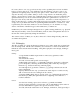
POEMS Parameters File Front-End Script POEMS.CMD foo.par CAD Export Utility foo.par.in Optimization Loop CAD File POSTPROC Orders File foo.orders FDTD Engine: FIDO + CLUSTER SCRIPT or TEMPEST FIDO Output File Postprocessor: POSTPROC RESULTS FIDO Input File EMPOST.EXE FIDO Field Files foo.par.out FIDO Log File foo.par.err foo.results Visualization System Bitmap Image Image Files Files Vis5D.EXE Vis5D Visualization Files Figure 2.
2. HOW POEMS WORKS 2.1. Program Organization The POEMS system consists of six parts: the front-end script (poems.
merit function, plus any binary file, list, or slice bitmaps requested. Doing this on each iteration takes little time and helps in supervising the run’s progress. (vi)Based on the computed merit function, update the optimization simplex. If convergence has occurred, exit. Otherwise, compute new values of the controlling variables for the next iteration and keep iterating. If the current point is the best so far, save all the bitmap, list, and mode files under another name.
from a linear to a logarithmic scale, change a colour palette, or something like that; simple changes like that are easily made directly to the generated file. EMPOST’s calling syntax is empost orders_file results_file The second argument is the name of a file that EMPOST produces, containing numerical results of the named orders, e.g. integrals, fluxes, mode matching coefficients, and so on. These are in the form of assignment statements, and are parsed by POEMS when postprocessing is completed.
2.6.1. Parallel Processing [Under construction] FIDO is a powerful and versatile simulation engine, which can compute simulations using inhomogeneous cubic grids on uniprocessors, symmetric multiprocessors (SMPs), and clusters tied together with TCP/IP. From the POEMS user’s point of view, SMPs act just like uniprocessors, except that an N-way SMP needs its work divided up into at least N chunks, and the load balancing is manual--usually it’s easy.
3. USING POEMS Everything in POEMS is case-insensitive. Case is preserved but not significant in file names; specifying two names equal except for case will cause the first to be overwritten in Windows and OS/2 but not in Linux. 3.1. Command Reference 3.1.1. poems Command-Line Options The calling syntax for POEMS is poems parmfile <- option1 >> where the options are one of DEBUG VERBOSE and RESTART.
FREQ LAMBDA Syntax: FREQ Syntax: LAMBDA Specify the frequency or free-space wavelength of the excitation sources (all will be the same). FREQ is an alternative to LAMBDA—use one or the other, but not both. Examples: FREQ 200*THz FREQ c/(1.464*700*nm) LAMBDA 1.55*micron LAMBDA 6.328e-7 FUNCTION /* 700 nm in fused SiO2 */ /* Communication wavelength */ /* He-Ne laser */ Define a user math function.
/* e.g. for a Thinkpad T23 laptop, /* Kukla--1.13 GHz PIII 127.0.0.1 localhost 1066 1 1.0 768 X86 OS/2 4.5 The port number is used for FIDO supervisory control, i.e. if this host is supervising N other hosts, those N connect to the supervisor using this port number. This port can be anything that doesn’t conflict with another service on the same cluster, but the unofficial "well-known" port for POEMS is 1066.
given name and field component. The parameters xsize, ysize, zsize are not macro parameters, but will be supplied from the current context when the macro is expanded. Note the string concatenation used to generate the file names. MACDEF FieldAll(kwd, fname)), /* Make I and Q field files /* with appropriate file names and symbolic limits FIELD variable=kwd xlo=0 xhi=xmax ylo=0 yhi=ymax , zlo=0 zhi=zsize phase=0.
Syntax: PRINT <"string"> .... RANDOMSEED Supply a seed to the pseudorandom number generator. Pseudorandom numbers are used only to choose starting points for the optimizer. The points visited by the optimizer for a given problem can be changed by choosing a different seed. Syntax: RANDOMSEED The value of must be in [0, 999,999,999], and its value is rounded to an integer before use.
Example: SIMULATOR /usr/local/tempest/tempest SIMULATOR rexx d:\poems\fido\fidossh.cmd $h $f TITLE Give a title to the run. This title is printed in each file, and is also used to generate names for the intermediate file and log file, and for the postprocessor orders file. No default. Syntax: TITLE Waveguide3a VERBOSE Turn on verbose output. Sometimes helpful in figuring out what’s going on. It’s sufficiently verbose that it’s probably best to redirect it to a file or a pager program such as less.
subdomain uses 6 sockets, attached to port, port+1,..., port+5, all of which must be unique on the given host, though there is nothing to stop different hosts from using the same port numbers. Port numbers must be between 0 and 65535, and it is usually best to use numbers greater than 16384. Syntax: SUBDOMAIN [host= port= , super=] BASICSTEP XRANGE YRANGE ZRANGE Specify the size of the cubical cells that make up the current subdomain.
materials are of this type: vacuum, air, glass, and plastics. Parameters: n, k (real and imaginary refractive index) Example: DEFINE matname= BlackGlass type=dielectric n=1.52 k=1e-3 Type metal Nonmagnetic dispersive material which may have negative dielectric constant at the frequency of interest, which is equivalent to having n < k, e.g. metals in the infrared. Other conductive materials can be modelled as conductor type.
Type PEC Type black Perfect conductor. All fields inside a PEC are zero. Sometimes useful for saving CPU cycles in regions where the fields are known to be zero, e.g. deep inside metal objects. Parameters: none 3.1.5. OBJECT Group Like all dimensions in POEMS, object dimensions are measured from edge to edge, as you would measure with calipers. All dimensions are correctly rounded to the nearest multiple of basicstep in the subdomain in which they occur.
If the two end faces are the same size and shape, all the curve shapes are equivalent. The end faces can be offset laterally, so that a fan statement can build a diagonal line. Parameters: matname taper taperpar xlo1 xhi1 ylo1 yhi1 zlo1 zhi1 xlo2 xhi2 ylo2 yhi2 zlo2 zhi2 GRATING Adds a planar grating with lines of rectangular cross-section. The line width and phase of the grating are arbitrary, and specified with user functions of the coordinate variables.
corners. This primitive is especially useful with plane wave illumination, where we want PMLs only on the front and back faces of the region. The wide face of the object must touch one of the faces of the simulation domain. The PML absorption directions will be the outward normals for the face, outward-directed face diagonals for the edges, and outward-directed body diagonals for the corners. If for some reason you call this with an ordinary material, it just adds a regular block.
3.1.6. SOURCE Group GAUSSIAN Produces a TEM00 Gaussian beam, centred at (x, y, z), with 1/e2 diameter width, whose axis is specified by the vector(kx, ky, kz), which can have any length. The E field is linearly polarized, with components (mag*Ex, mag*Ey, mag*Ez). Circular or elliptical polarizations can be synthesized by using two with different phases. In this release, orientation must be XY, because tempest can’t handle plane waves whose source locus isn’t perpendicular to z.
POINT Adds a linearly-polarized point electric dipole source at the given position. Point sources whose polarization is not x, y, or z (diagonally, circularly, or elliptically polarized) can be implemented as two or three point sources with appropriately chosen magnitude and phase. Parameters: x y z Ex Ey Ez mag phase 3.1.7. COMMAND Group COMPUTE Supply control parameters to FIDO/TEMPEST.
FIELD Tells tempest to produce a field file containing the specified field variable at each point. Parameters: variable xlo xhi ylo yhi zlo zhi x y z file phase state 3.1.9. POSTPROCESS Group CAD Produces a .ctxt (2-D) or 2-D or 3-D DXF file of the entire simulation domain, suitable for importation into a CAD program, e.g. for numerically controlled machining, photomask generation, or documentation. In a 3-D DXF file, each block in the simulation domain becomes a set of six 3DFACE entities. In a .
FARFIELD Computes the far-field limit of the fields at a given plane, specified as xlo ≤ x ≤ xhi, ylo ≤ y ≤ yhi, zlo ≤ z ≤ zhi. Because this range must specify a plane, the upper and lower limits of one axis must be the same to within basicstep/2. The coordinates will be correctly rounded to integral numbers of cells. We assume that the fields propagate through an infinite half-space of refractive index n (which obviously must be lossless).
LIST Stores a list of field values as ASCII floating point numbers, suitable for reading into a spreadsheet or a plotting program such as GNUPLOT. The row-column arrangement of a 3-dimensional list file depends on the value of orientation. Coordinate axes are always taken in cyclic order, with the leftmost position in the first line corresponding to the minimum of all coordinates; in a 2-D list in XY orientation (perpendicular to Z), columns correspond to the x coordinate and rows to the y coordinate.
Parameters: name xinside yinside zinside function exi exq eyi eyq ezi ezq xlo xhi ylo yhi zlo zhi xfocus yfocus zfocus xNA yNA zNA NA direction MOVIE Produces an animated one-cycle GIF of N frames, over the given plane. Parameters:file orientation xlo xhi ylo yhi zlo zhi dt frames variable Not implemented in this release. MOVIE3D Produces an interactive Vis5D animation of up to 9 field variables.
DISSIPATION Power dissipation density , -∇ S (the Poynting vector). Normalized to the volume of one cell, so that volume integrals of this quantity give the correct power dissipation inside the region. Parameters: name xlo xhi ylo yhi zlo zhi file xinside yinside zinside SLICE Produce a bitmap of variable over the given domain, with control over the colour palette and the scale. Variables are always taken in cyclic order, i.e. x, y, z, x, y, z,...
where level, R, G, and B are integers between 0 and 255, inclusive. The level column represents the signal level, and R, G, and B are the usual RGB colour components. Choices of curve are linear, gamma, logarithmic, and MuLaw. The linear curve spaces the palette entries out evenly, with the maximum value in the picture being 255 and the minimum, 0. The gamma curve first takes the square root of the absolute value of the variable, restores the sign, and spaces out the result evenly.
supplied, guess N+2 overwrites guess 1, and so on. You can supply a pre-computed value for the penalty or merit function, by including merit= or penalty= in the GUESS statement. While this can save valuable time, it must be used with care, because POEMS will trust the value you give it. If the value is stale or otherwise incorrect, this will interfere with the optimization.
Syntax: MERIT OR PENALTY Example: PENALTY 100*(OutputFlux/InputFlux - 1) PARAMETERS Defines quantities to guide the optimizer. The number of function evaluations (i.e., tempest runs) per restart will not exceed iterations, convergence will be declared when the penalty function value in all the simplex points is within tolerance of the best value, and the optimizer will be restarted restarts times after converging or running out of iterations.
3.2. The Computational Domain 3.2.1. Symmetry Many technologically useful devices have a periodic structure. The periodic boundary conditions assumed by POEMS are a natural fit to such structures, which can be simulated very efficiently. This happens automatically if you leave out the absorbers on the sides facing the periodic direction. Almost as many devices exhibit symmetry planes.
Another way of stating this is that if a symmetry plane is like a mirror, then we’d expect that a block pushed right up against it would look like two blocks. With POEMS, we have to think of it as pushing a block up to and halfway through the mirror, so it still looks like one block. A one-block layer at the symmetry axis unfolds to one block, a two-block layer unfolds to three blocks, and in general N blocks unfold to 2N-1 blocks.
3.3.1. Perfectly-Matched Layers PMLs are fictitious anisotropic materials that (usually) absorb whatever radiation falls on them from pre-specified directions. They work extremely well when they work at all, which isn’t 100% of the time. PMLs don’t absorb in every direction, so different parts of the domain need different PMLs. This is such a pain that POEMS makes a valiant effort to automate it for you.
source is therefore an oscillating dipole. FDTD codes model a dipole as a single-cell source whose E field oscillates in time, just as you’d expect. Unfortunately, only linearlypolarized sources are supported because only a single point source can occupy a cell. This restriction is not essential, and may be removed in a future release. The other problematical thing about point sources is normalization.
FDTD codes use periodic boundary conditions. Fields leaving through one side will magically reappear coming from the other, which may lead to divergences if you don’t put in absorbers of some sort. Sloppy absorber design may lead to fields travelling many, many periods, leading to anomalously slow convergence. Figure 2.4 is an example of a divergence due to PMLs used with plane wave sources. Note that the divergence looks electrostatic—the wavelength is far too short to propagate.
3.5.3. BEAM SOURCES Beam sources are made up of sums of plane waves. They share the unidirectional property of plane sources. This is sometimes useful in waveguide simulations, because you can bounce the wave off a mirror at the far end and look at the field coming backwards through the plane wave surface. Since all of this field has travelled twice the length of the waveguide, it can make a good approximation of the waveguide mode. This is where the mode file used in 3.5.4 came from. 3.5.4.
3.6. Optimization There are powerful techniques for finding the minimum of smooth functions in a few function evaluations, an important consideration when the merit function requires minutes to hours for each iteration. There are robust techniques for finding the minimum of functions that are noisy, discontinuous, or otherwise badly behaved, which our simulation results tend to be.
FLUX FLUX name=PwrIn xlo=0 xmax=10*um ylo=0 ymax=12*um z=zSource+1*um, zinside = zSource+2*um xinside = xsize/2 yinside=ysize/2 name=PwrIn xlo=0 xmax=10*um ylo=0 ymax=12*um z=zOutput, zinside = zSource+2*um xinside = xsize/2 yinside=ysize/2 END OPTIMIZE PENALTY (PwrIn-PwrOut)/PwrIn ... END b.
3.6.2. Worked Example: Optimizing a V Antenna Thermodynamics dictates that the total power an antenna can deliver to its terminals when excited by isotropic thermal radiation cannot be larger than kT per hertz (otherwise you could put a hot resistor at the feed point, point the antenna at a colder object, and have the resistor get hotter spontaneously).
Figure 2.14 Optimized V antenna: power dissipation density. maximum at the feed point.
3.6.3. Worked Example: Doped Silica Waveguide Mode In simulating waveguide devices, the first requirement is to have a source that produces a pure waveguide mode. Sometimes a Gaussian beam is sufficient, but often it is not, especially when small reflections or phase shifts are important. Analytical solutions are not often available for the modes of real dielectric guides, so a numerical procedure is of more general use.
fs as = = ps/1000 fs/1000 kHz MHz GHz THz EHz = = = = = 1000 1000*kHz 1000*MHz 1000*GHz 1000*THz pi twopi deg degree rad cycle = = = = = = 3.141592653589793 2*pi pi/180 deg 1.0 twopi c mu0 eps0 = = = 299792458 4*pi*1e-7 1/(c*c*mu0) 3.7.1. Reserved Names Figure 2.16 Detail of the launch end. Note the unidirectional character of the Gaussian beam source, and the weak reflected field leaking back through the illumination plane after travelling about 110 µm.
Figure 2.17: Detail of the CAD output for one iteration of the glass ridge waveguide to free space coupler. 3.8. Predefined Mathematical Functions 3.8.1. Arithmetic Operators The user-facing part of POEMS is implemented in REXX, so the arithmetic and logical operators and many of the simpler mathematical functions are native REXX constructs, and have REXX syntax and semantics.
Also, REXX does not distinguish between integer and floating-point numbers. It isn’t that it uses floats for everything—internally REXX uses arbitrary-precision arithmetic. 3.8.2. Logical Operators > (greater than) < (less than) ≥ (greater or equal) ≤ (less or equal) <> (unequal) \ (not) 3.8.3. ABS Returns the absolute value of . Syntax: abs() 3.8.4. ACOS Returns the radian angle in [0, 2π) whose cosine is .
3.8.10. ATAN2 Returns the radian angle in (-π, π] whose tangent is /, and which is in the correct quadrant. Syntax: atan2(, ) 3.8.11. CEIL Returns the smallest integer that is at least as large as the argument (i.e., round towards +∞). More useful than integer truncation, since it Does The Right Thing with negative arguments. Syntax: ceil() 3.8.12. COS Returns the cosine of radian argument .
nright=number of places to the right of the decimal exptol=trigger for exponential notation nexp=number of places in the exponent FORMAT(’12345.73’,,,2,2) FORMAT(’12345.73’,,3,,0) FORMAT(’1.234573’,,3,,0) FORMAT(’12345.73’,,,3,6) FORMAT(’1234567e5’,,3,0) → → ’1.234573E+04’ → ’1.235E+4’ → ’1.235’ → ’12345.73’ ’123456700000.000’ 3.8.19. INTEGRAL Computes the 1-dimensional integral of user function f from xlo to xhi. Just a stub at present. Syntax: INTEGRAL(f, xlo, xhi) 3.8.20. LN Natural logarithm.
3.8.26. RANDOM Interface to the REXX pseudorandom number generator. Returns a pseudorandom integer from > to , inclusive, and optionally re-seeds the generator with , evaluated and rounded to an integer. Default values : , , ) 3.8.27.
3.9. Analytical Pupil Functions POEMS knows about the following analytical pupil functions: GAUSSIAN AIRY FLATTOP TEM00 Gaussian beam Uniform circular disc pupil function, resulting in an Airy function at the focus E=2J1(krNA)/(krNA), the jinc function. Pupil function is a jinc times a circularly-symmetrical Hamming window, resulting in a focused beam with a flat top and smoothly sloping sides. The actual pupil function is E(u,v)=2(0.54+0.46cos(πρ))J1(6πρ)/(6πρ), where ρ=(u2+v2)1/2/NA. 3.10.
A. TEMPEST and General FDTD Information relies on the finite-difference time domain algorithm of Yee for its calculations. The Yee algorithm simulates the Maxwell curl equations directly, on two interpenetrating grids, half a step apart in each axis: one for H and one for E.
TEMPEST uses the following code for choosing the time step (MAXDIMENSION is 3): dt=(dx/(C/min_index*sqrt((DOUBLE)(MAXDIMENSION)))) ; period_step=ceil((DOUBLE)((2.0*PI)/(omega*dt))) ; period_step+=2; i=period_step%4; if (i!=0) period_step=(period_step+4-i) ; dt=((2.
Appendix A.: V-Antenna Optimization Run This appendix contains a complete worked example of a three-parameter optimization of a 3-D simulation. The device to be optimized is a V-dipole antenna made of gold, working in free space at a wavelength of 1.58 µm. The parameters being optimized are the length (in X) and rake (in Z) of the arms of the antenna, and the load resistance applied to the output terminals. The merit function is the power dissipated in the load.
A.1. POEMS INPUT: DIPOLE2I.PAR (This is what you write.) /* /* /* /* /* /* /* Dipole2I.par: Simple test using a 10-micron cube of free space with PML boundaries Uses poems and tempest 6.0 by Phil Hobbs, November 24, 2003 GLOBAL comment COMMENT dipole2i: comment Optimization of a V antenna for maximum power absorption from free space comment Parameters optimized: length and rake of antenna, load impedance comment comment simulator tempest lambda 1.58*um title Dipole2I postprocessor empostpr.
/* Fundamental dimensions */ set set set set set set set set set set step=um/20; Tpml = 8*step xsize=5.1*um ysize=xsize zsize=6.2*um; dipoleheight=0.2*um; dipolethickness=0.30*um; phi=0; /* phase of excitation */ ky0=step/lambda; kx0=0; /* direction of plane wave */ set set set set loadlength=2*step; loadThickness=dipolethickness loadheight=dipoleheight Zvertex=zsize-Tpml-loadthickness/2-1.5*um /* back end of load 1.5 um from PML */ set set set set set set set DipoleLengthUM = 1.
DEFINE matname= Load type=dielectric n=n_load k=k_load END WORLD SUBDOMAIN ALL XRANGE 0 xsize YRANGE 0 ysize ZRANGE 0 zsize BASICSTEP step BOUNDARY ymax illum BOUNDARY xmin illum BOUNDARY zmax illum END OBJECT /* Absorber around the outside of the domain */ HOLLOWBOX matname=AirPML xlo=0 xhi=xsize ylo=0 yhi=ysize zlo=0 zhi=zsize thickness=Tpml /* Air filling all space inside PML */ BLOCK matname=Air xlo=Tpml xhi=xsize-Tpml ylo=Tpml yhi=ysize-Tpml , zlo=Tpml zhi=zsize-Tpml /* Dipole FAN matname=PCL taper=
zlo2 = Zvertex-DipoleThickness/2 zhi2= Zvertex+DipoleThickness/2 FAN matname=PCL taper=linear taperpar=0 , xlo1 = (xsize+LoadLength)/2 xhi1=(xsize+LoadLength)/2 , ylo1 = (ysize-DipoleHeight)/2 yhi1=(ysize+DipoleHeight)/2, zlo1 = Zvertex-DipoleThickness/2 zhi1= Zvertex+DipoleThickness/2, xlo2 = (xsize+DipoleLengthUM*um)/2 xhi2=(xsize+DipoleLengthUM*um)/2, ylo2 = (ysize-DipoleHeight)/2 yhi2=(ysize+DipoleHeight)/2, zlo2 = Zvertex-ZRakeUM*um-DipoleThickness/2 zhi2= Zvertex-ZRakeUM*um+DipoleThickness/2 /* Load B
FIELD variable=Ey xlo=0 xhi=xsize ylo=0 yhi=ysize zlo=0, zhi=zsize phase=0.25*cycle state=steady file=Dipole2I_eyq FIELD variable=Ez xlo=0 xhi=xsize ylo=0 yhi=ysize zlo=0, zhi=zsize phase=0 state=steady file=Dipole2I_ezi FIELD variable=Ez xlo=0 xhi=xsize ylo=0 yhi=ysize zlo=0, zhi=zsize phase=0.
END POSTPROCESS AMPLEX xlo=0 xhi=xsize ylo=0 yhi=ysize zlo=0 zhi=zsize file=Dipole2I_AmplEx PHASEEX xlo=0 xhi=xsize ylo=0 yhi=ysize zlo=0 zhi=zsize file=Dipole2I_PhaseEx FARFIELD xlo=Tpml xhi=xsize-Tpml ylo=Tpml yhi=ysize-Tpml zlo=zsize-Tpml-step, zhi=zsize-Tpml-step file=Dipole2IFF1 name=ff2 POYNTINGY xlo=0 xhi=xsize ylo=0 yhi=ysize zlo=0 zhi=zsize file=Dipole2I_py POYNTINGX xlo=0 xhi=xsize ylo=0 yhi=ysize zlo=0 zhi=zsize file=Dipole2I_px POYNTINGZ xlo=0 xhi=xsize ylo=0 yhi=ysize zlo=0 zhi=zsize file=Dipo
zhi = zsize-Tpml-step , xinside=xsize/2 yinside=ysize/2 zinside=zsize/2 FLUX name=MiddleFlux , /* crossing the middle (z=zsize/2) xLo = Tpml , xhi = xsize-Tpml, yLo = Tpml , yhi = ysize-Tpml , zlo = zsize/2 , zhi = zsize/2 , xinside=xsize/2 yinside=ysize/2 zinside=zsize INTEGRAL name=diss variable=dissipation, xlo=(xsize-LoadLength)/2 xhi=(xsize+LoadLength)/2, ylo = (ysize-LoadHeight)/2 yhi=(ysize+LoadHeight)/2, zlo = Zvertex-LoadThickness/2 zhi=Zvertex+LoadThickness/2, SLICE orientation=xy variable=indexn
SLICE orientation=zx variable=PoyntingZ , xlo=0 xhi=xsize , ylo=ysize/2 yhi=ysize/2, zlo=0 zhi=zsize, file=Dipole2IPZ_ZX.bmp phase=0 palette=redblue SLICE orientation=xy variable=PoyntingX , xlo=0 xhi=xsize, ylo=0 yhi=ysize, zlo=zsize/2 zhi=zsize/2, file=Dipole2IPX_XY.bmp phase=0 palette=redblue SLICE orientation=zx variable=PoyntingX , xlo=0 xhi=xsize , ylo=ysize/2 yhi=ysize/2, zlo=0 zhi=zsize, file=Dipole2IPX_ZX.
file=Dipole2IDiss_XY.bmp palette=redblue SLICE orientation=zx variable=Dissipation , xlo=0 xhi=xsize , ylo=ysize/2 yhi=ysize/2, zlo=0 zhi=zsize, file=Dipole2IDiss_ZX.bmp palette=redblue SLICE orientation=zx variable=Dissipation , xlo=0 xhi=xsize , ylo=ysize/2 yhi=ysize/2, zlo=0 zhi=zsize, file=Dipole2IDiss_ZXmu.bmp palette=redblue curve=mulaw SLICE orientation=xy variable=PhaseEx , xlo=0 xhi=xsize, ylo=0 yhi=ysize, zlo=zsize/2 zhi=zsize/2, file=Dipole2IPhaseEx_XY.
ylo=ysize/2 yhi=ysize/2, zlo=0 zhi=zsize, file=Dipole2IExQ_ZX.
A.2. tempest Input File: DIPOLE2I.PAR.IN This file is machine-generated. The real one is much larger than this—56 pages’ worth of point_source statements have been snipped out here. The only reason to read this file at all is to check that, e.g. there are no gaps between different layers of material, and this is probably better done using the DXF export utility and DXF file viewer.
/* /* /* /* /* /* /* /* /* /* /* /* /* /* /* /* /* /* /* /* /* /* /* /* /* /* /* /* /* /* /* /* ************************************************************************ ************************************************************************ \\KUKLA\X:\frontend\dipole2i.par.in: tempest Input file generated by Optimizing Simulator Framework Tool \\KUKLA\X:\frontend\poems.cmd from Parameter file: \\KUKLA\X:\frontend\dipole2i.par Script version 0.
rectangle rectangle rectangle rectangle rectangle rectangle rectangle rectangle rectangle rectangle rectangle rectangle rectangle rectangle rectangle rectangle rectangle rectangle rectangle rectangle rectangle rectangle rectangle rectangle rectangle rectangle rectangle rectangle node node node node node node node node node node node node node node node node node node node node node node node node node node node node 90 0 90 8 8 8 8 0 90 0 90 0 90 0 90 8 34 35 36 38 39 40 41 42 43 45 46 47 98 8 98 90 90 9
... err_tol 2.000000E-04 max_cycle 8 plot refractive node 0 97 0 97 0 119 plot ex steady 0.000000 node 0 97 0 plot ex steady 0.250000 node 0 97 0 plot ey steady 0.000000 node 0 97 0 plot ey steady 0.250000 node 0 97 0 plot ez steady 0.000000 node 0 97 0 plot ez steady 0.250000 node 0 97 0 plot hx steady 0.000000 node 0 97 0 plot hx steady 0.250000 node 0 97 0 plot hy steady 0.000000 node 0 97 0 plot hy steady 0.250000 node 0 97 0 plot hz steady 0.
DIPOLE2I_EYI DIPOLE2I_EYQ DIPOLE2I_EZI DIPOLE2I_EZQ DIPOLE2I_HXI DIPOLE2I_HXQ DIPOLE2I_HYI DIPOLE2I_HYQ DIPOLE2I_HZI DIPOLE2I_HZQ DIPOLE2I_REFRACTIVE 0.00000 4.90000E-06 0.00000 4.90000E-06 0.00000 6.00000E-06 DISS 1 NULL_EXI NULL_EXQ NULL_EYI NULL_EYQ NULL_EZI NULL_EZQ NULL_HXI NULL_HXQ NULL_HYI NULL_HYQ NULL_HZI NULL_HZQ NULL_INDEXN 2.40000E-06 2.35000E-06 3.80000E-06 2.50000E-06 2.55000E-06 4.
NULL_EXI NULL_EXQ NULL_EYI NULL_EYQ NULL_EZI NULL_EZQ NULL_HXI NULL_HXQ NULL_HYI NULL_HYQ NULL_HZI NULL_HZQ NULL_INDEXN 4.00000E-07 4.00000E-07 5.55000E-06 MIDDLEFLUX 1 NULL_EXI NULL_EXQ NULL_EYI NULL_EYQ NULL_EZI NULL_EZQ NULL_HXI NULL_HXQ NULL_HYI NULL_HYQ NULL_HZI NULL_HZQ NULL_INDEXN 4.00000E-07 4.00000E-07 3.00000E-06 4.50000E-06 4.50000E-06 5.55000E-06 4.50000E-06 4.50000E-06 3.
ARRAY PHASEEX 0.00000 4.90000E-06 0.00000 4.90000E-06 0.00000 6.00000E-06 0.00000 0.00000 0.00000 0.00000 0.00000 0.00000 0.00000 0.00000 0.00000 0.00000 0.00000 0.00000 -4.90000E-06 -4.90000E-06 -6.00000E-06 POSTPROC.2.COMPARISONDOMAIN POSTPROC.2.PARMSTRING DIPOLE2I_PHASEEX /* /* /* /* /* /* /* /* /* /* /* /* /* FF2 ARRAY FARFIELDS 4.00000E-07 4.50000E-06 4.00000E-07 4.50000E-06 5.55000E-06 5.55000E-06 0.00000 0.00000 0.00000 0.00000 0.00000 0.00000 0.00000 0.00000 0.00000 0.00000 0.00000 0.00000 -4.
POSTPROC.5.COMPARISONDOMAIN POSTPROC.5.PARMSTRING DIPOLE2I_PX /* /* /* Domain for comparison (e.g. modematch) Order-dependent parameter string (e.g. name of calculated mode function) Output file for calculated data POSTPROC.6.NAME ARRAY POYNTINGZ 0.00000 4.90000E-06 0.00000 4.90000E-06 0.00000 6.00000E-06 0.00000 0.00000 0.00000 0.00000 0.00000 0.00000 0.00000 0.00000 0.00000 0.00000 0.00000 0.00000 -4.90000E-06 -4.90000E-06 -6.00000E-06 POSTPROC.6.COMPARISONDOMAIN POSTPROC.6.
0.00000 0.00000 0.00000 0.00000 0.00000 0.00000 0.00000 0.00000 2.45000E-06 2.45000E-06 OUTPUTFACETFLUX POSTPROC.9.PARMSTRING NULL 0.00000 3.00000E-06 /* /* /* /* /* /* /* /* xfocus, yfocus, zfocus( for mode computation) ExI, ExQ (V/m) (for mode computation) EyI, EyQ (V/m) (for mode computation) EzI, EzQ (V/m) (for mode computation) xInside yInside zInside (metres)--coordinates of a point ’inside’ the surface Domain for comparison (e.g. modematch) Order-dependent parameter string (e.g.
SLICE POYNTINGZ 0.00000 4.90000E-06 0.00000 4.90000E-06 3.00000E-06 3.00000E-06 0.00000 0.00000 0.00000 0.00000 0.00000 0.00000 0.00000 0.00000 0.00000 0.00000 0.00000 0.00000 -4.90000E-06 -4.90000E-06 -6.00000E-06 POSTPROC.13.COMPARISONDOMAIN 0 LINEAR GREY DIPOLE2IPZ_XY0.
POSTPROC.16.COMPARISONDOMAIN 0 LINEAR GREY DIPOLE2IPX_ZX0.BMP /* /* /* POSTPROC.17.NAME SLICE AMPLEX 0.00000 4.90000E-06 0.00000 4.90000E-06 3.05000E-06 3.05000E-06 0.00000 0.00000 0.00000 0.00000 0.00000 0.00000 0.00000 0.00000 0.00000 0.00000 0.00000 0.00000 -4.90000E-06 -4.90000E-06 -6.00000E-06 POSTPROC.17.COMPARISONDOMAIN 0 LINEAR GREY DIPOLE2IAMPLEX_XY0.
0.00000 0.00000 0.00000 0.00000 0.00000 0.00000 0.00000 0.00000 0.00000 -4.90000E-06 -4.90000E-06 -6.00000E-06 POSTPROC.20.COMPARISONDOMAIN 0 LINEAR GREY DIPOLE2IDISS_ZX0.BMP /* /* /* /* /* /* /* /* xfocus, yfocus, zfocus( for mode computation) ExI, ExQ (V/m) (for mode computation) EyI, EyQ (V/m) (for mode computation) EzI, EzQ (V/m) (for mode computation) xInside yInside zInside (metres)--coordinates of a point ’inside’ the surface Domain for comparison (e.g.
SLICE EX 0.00000 4.90000E-06 2.45000E-06 2.45000E-06 0.00000 6.00000E-06 0.00000 0.00000 0.00000 0.00000 0.00000 0.00000 0.00000 0.00000 0.00000 0.00000 0.00000 0.00000 -4.90000E-06 -4.90000E-06 -6.00000E-06 POSTPROC.24.COMPARISONDOMAIN 1.57079632679 LINEAR GREY DIPOLE2IEXQ_ZX0.
A.4. Run Results: DIPOLE2I.SIMPLEX This file contains a summary of the optimizer’s progress, including everything you need to start another run where this one left off. If you need to stop and restart the simulation, the last simplex can be cut and pasted into GUESS statements in the input file. That way no work is wasted. Starting a new run at 1 Jun 2003 08:50:29 0.0000008 80 0.00000140 -30566.31 5.699520E-007 9.940356E+001 1.511401E-006 -49632.84 .2000000E-006 1.290000E+002 1.000000E-006 -20316.57 7.
Contracting by 0.5 in 1D. 1-D shrink unsuccessful. Condition number is 5.11775473802E+16Should be below 10**5 Shrinking down around best point (WILL TAKE A WHILE) 0.00000064767135 98.83191 0.000001519205 Penalty = -49145.21 0.00000069266248611 90.849532778 0.00000152214633334 Penalty = -43884.55 0.000000883423566665 77.7563866665 0.0000017351705 Penalty = -25176.17 ZRAKE= 5.699520E-07 ZL= 9.940356E+01 DIPOLELENGTH= 1.511401E-06 penalty ZRAKE= 6.476714E-07 ZL= 9.883191E+01 DIPOLELENGTH= 1.
Reflecting through centroid. Contracting by 0.5 in 1D. ZRAKE= 5.538816E-07 ZL= 1.040048E+02 ZRAKE= 5.654595E-07 ZL= 1.018839E+02 ZRAKE= 6.053845E-07 ZL= 1.002980E+02 ZRAKE= 5.699520E-07 ZL= 9.940356E+01 DIPOLELENGTH= DIPOLELENGTH= DIPOLELENGTH= DIPOLELENGTH= 1.492537E-06 1.459659E-06 1.503535E-06 1.511401E-06 penalty penalty penalty penalty =-5.174051E+04 =-5.138234E+04 =-5.132064E+04 =-4.963284E+04 Reflecting through centroid. Contracting by 0.5 in 1D. ZRAKE= 5.538816E-07 ZL= 1.040048E+02 ZRAKE= 5.
Reflecting through centroid. Contracting by 0.5 in 1D. ZRAKE= 5.538816E-07 ZL= 1.040048E+02 ZRAKE= 5.654595E-07 ZL= 1.018839E+02 ZRAKE= 6.053845E-07 ZL= 1.002980E+02 ZRAKE= 5.747536E-07 ZL= 1.019791E+02 DIPOLELENGTH= DIPOLELENGTH= DIPOLELENGTH= DIPOLELENGTH= 1.492537E-06 1.459659E-06 1.503535E-06 1.486061E-06 penalty penalty penalty penalty =-5.174051E+04 =-5.138234E+04 =-5.132064E+04 =-4.965101E+04 Reflecting through centroid. Contracting by 0.5 in 1D. ZRAKE= 5.538816E-07 ZL= 1.040048E+02 ZRAKE= 5.
ZRAKE= ZRAKE= ZRAKE= ZRAKE= 5.538816E-07 5.907142E-07 5.930227E-07 5.823060E-07 ZL= ZL= ZL= ZL= 1.040048E+02 1.007803E+02 1.016992E+02 1.009124E+02 DIPOLELENGTH= DIPOLELENGTH= DIPOLELENGTH= DIPOLELENGTH= 1.492537E-06 1.484533E-06 1.470509E-06 1.481122E-06 penalty penalty penalty penalty =-5.174051E+04 =-4.860518E+04 =-4.860450E+04 =-4.834583E+04 Reflecting through centroid. Contracting by 0.5 in 1D. ZRAKE= 5.538816E-07 ZL= 1.040048E+02 ZRAKE= 5.907142E-07 ZL= 1.007803E+02 ZRAKE= 5.930227E-07 ZL= 1.
ZRAKE= ZRAKE= ZRAKE= ZRAKE= 80 5.538816E-07 5.579771E-07 5.559206E-07 5.430786E-07 ZL= ZL= ZL= ZL= 1.040048E+02 1.041947E+02 1.046504E+02 1.053899E+02 DIPOLELENGTH= DIPOLELENGTH= DIPOLELENGTH= DIPOLELENGTH= 1.492537E-06 1.490018E-06 1.486328E-06 1.496543E-06 penalty penalty penalty penalty =-5.174051E+04 =-5.173870E+04 =-5.173462E+04 =-5.149381E+04 Reflecting through centroid. Contracting by 0.5 in 1D. ZRAKE= 5.538816E-07 ZL= 1.040048E+02 ZRAKE= 5.579771E-07 ZL= 1.041947E+02 ZRAKE= 5.
Appendix B.: Configuration An axiom of programming is that in setting up a new development system, once you can get "Hello, World" to compile, link, and run, you’re most of the way there. With POEMS, the equivalent point is when you have the REXX interpreter working and VIS5D’s demos running in X. If you’re new to FDTD simulation, you may encounter some puzzling behaviour, especially numerical divergences if you try to pack things in too tightly. This appendix is intended to make these things easier. B.1.
B.1.2. tempest limitations a. Off-axis plane waves. Symmetrical domains of course must have symmetrical illumination. The TEMPEST approach is to forbid such domains to have off-axis plane waves applied to them. The other approach would have been to double each plane wave source, so that their result was symmetric, which would be preferable. Since the xxBEAM source statements are implemented as sums of plane waves, we can’t use them on symmetric domains. Use mode sources instead.
Big PMLs cost a great deal of memory and computation time, at least triple that required by ordinary materials. This is not improved by overwriting the PML blocks with other materials, so if you were considering filling all space with PML and writing other things over it, don’t. Have a look at the HOLLOWBOX and TILEDPLANE statements for alternatives. Don’t use a wavelength that is an exact multiple of the cell size. This will often slow convergence. Once FIDO/TEMPEST starts to page, it’s all over.
rem PMX SET DISPLAY=localhost:0 SET XFFILES=E:\MPTN\X11 rem End PMX rem XFree86 4.2 set x11root=f: set xserver=f:\xfree86\lib\xfree86.exe; set home=f:\hobbs set display=localhost:0.0 set manpath=f:\xfree86\man\man1;f:\xfree86\man\man3;f:\xfree86\man\man4;f:\xfree86\ man\man7;f:\emx\man; device=f:\xfree86\lib\xf86sup.sys set termcap=f:/emx/etc/termcap.dat set user=hobbs set logname=hobbs rem End XFree86 4.2 B.3.2.
d. Adjustments to the postprocessor: (i) Figure out how to eliminate the spurious negative dissipations at the edges of material blocks; (ii) Optionally produce bitmaps and mode files unfolded along the symmetry planes. This will make the bitmaps easier to read and will make modefile sources more flexible. e. Allow modefile sources to have a different cell size than the current simulation. We’re summing over several-block regions anyway, so there’s no reason we can’t interpolate as well. f.
compute the actual line width. This is more difficult when the limits are complicated. I hope that experience will show how important this is in practice. e. The version of TEMPEST we’re using is a uniprocessor implementation, so it can’t yet be used with grid computing. POEMS’s own FDTD engine is currently in the alpha stage--it produces correct simulations using collections of point sources and materials with n>k (i.e. dielectrics and normal metals at low frequencies).
Appendix C. Multiprocessing POEMS works seamlessly on uniprocessors and symmetrical multiprocessors (SMPs) that share a single memory image, as in machines using N-core CPUs or multiple CPU chips in a single box. In addition, it works on cluster machines with any degree of coupling. &po. uses a frontend script, poems.cmd, to The basic architecture of &po.
INDEX y iry pattern 21 A Antenna 1, 39, 40, 45, 51, 52, 63, 65 BASICSTEP 16, 18, 24, 54, 62 Boundary 7, 15, 19, 29, 31, 33-35, 54 C++ 7, 43 Conductor 2, 16-18, 51 Constants 41, 48 Convergence 7, 22, 30, 35, 49, 82, 83 Curve 18-20, 27, 28, 60 Cylinder 20 Debug 10, 52 Decimate 22 Dielectric 16-18, 41, 51, 53, 54 Dielectric constant 17 Dissipation 2, 26, 27, 38, 40, 49, 57, 58-60, 69, 72 Divergence 34, 35, 81 Domain 3, 7, 15, 16, 18-20, 22, 23, 27, 31-34, 49, 54, 62, 67, 68-74, 81, 82, 84, 85 DXF File (Autoca
Periodic boundary conditions 31, 34, 35 Philosophy 2 Pistor, Tom 3 Plane wave 1, 20, 21, 32, 34-36, 41, 51, 53, 82, 84, 86 Point source 34 Poynting vector 24, 26, 27, 36, 39, 49, 86 Process priority 81 Programmable Optimizing Electromagnetic Simulator (POEMS) iii, 1-10, 12-16, 18, 20, 21, 23, 24, 26, 27, 29, 31-34, 36, 37, 43, 48, 49, 51, 52, 62, 63, 65, 67-73, 81, 83, 84-87 Pupil function 21, 25, 34, 48 Refractive index 17, 22, 24-26, 39 Reserved names 42 REXX language 6, 7, 11, 13, 15, 43, 44, 45, 47, 81,