HP MLIB User's Guide Vol. 2 7th Ed.

540 HP MLIB User’s Guide

Associated documentation

The following documents provide supplemental material for this chapter:

Brigham, E.O. The Fast Fourier Transform. Englewood Cliffs, NJ:

Prentice-Hall, Inc. 1974.

Rabiner, L.R., and B. Gold. Theory and Application of Digital Signal Processing.

Englewood Cliffs, NJ: Prentice-Hall, Inc. 1975.

Van Loan, C. Computational Frameworks for the Fast Fourier Transform.

Philadelphia: Society for Industrial and Applied Mathematics, 1992.

What you need to know to use these subprograms

Strictly speaking, an FFT is not a type of transform but a class of algorithms for

efﬁciently computing the discrete Fourier transform (DFT).

Although the DFT is deﬁned for any number of data points, the VECLIB FFT

subprograms have the best performance when the number of points is

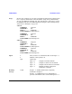
restricted to certain forms. For optimal performance, the number of points in

each direction should be a product of powers of 2, 3, and 5:

Problem sizes not of this form may take approximately ten times longer to

execute than similar idealized problem sizes.

In addition, for real-to-complex and complex-to-real, DFTs should also be even

for best performance.

While this restriction may limit the use of the subprograms, the gain in speed is

enormous. You can frequently adapt your data set for better performance by

augmenting it with enough zero-value data points to reach the next acceptable

number of points. Doing so slightly changes the problem, which may or may not

be important. For example, adding zero-value points to a time series changes

the implied sampling frequency, but adding zero-value points to data sets

before using FFT subprograms to compute convolutions does not change the

result.

,, 0.≥,=