Providing Open Architecture High Availability Solutions

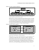
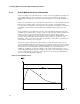
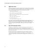
The trend of the ‘a’ line depicts the results of a hyper-exponential model [lapr92] that is also

backed by typical field data. It shows that systems typically peak in their unavailability shortly

after deployment, then, through reliability growth (defect removal), eventually stabilize near their

expected reliability level (c). The ‘b’ line represents the pessimistic reliability prior to defect

removal and reliability growth. The ‘c’ line represents the optimistic reliability after reliability

growth has taken place.

The ability to model the reliability and availability of a system taking into account reliability

growth is a relatively complex topic beyond the scope of this paper, however they can be

approximated by a statistical estimation. Details on this can be found in Laprie’s ‘Dependability:

Basic Concepts and Terminology [Lapr92].

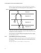
In that example, the availability of a system is given by the ratio of non-failed components at time t

to total number of components in the set. Integrated over time, the average gives an approximation

of the availability of the system from its time origin. The intervals or quantization of t over which

the availability is measured sets the granularity of observed availability. This estimation is a

passive appraisal of availability. That is, it is a simple way of expressing the observed availability

of a system once it is commissioned. An active model, like the one suggested by Laprie, offers the

ability to analytically estimate system availability prior to its commissioning [Lapr92]. While this

is only a model, it is one of the responsible ways in which system engineers can increase their

confidence and help reduce the risks in their ability to design and deploy highly-available systems.

3.5 Redundancy

Almost all hardware fault management techniques utilize redundancy, so it is helpful to expand this

further. Redundancy is generally classified into three basic types:

1. Spatial, which consumes space. This involves provisioning of more resources to provide a

service than would otherwise be needed – the extra resources are used when a primary

resource fails.

2. Temporal, which consumes time. An example of temporal redundancy is the ACK/NAK

method used by many protocols. A failure of reception causes the message to be repeated,

which is the redundancy, while the penalty is that of time.

3. Structural, sometimes called contextual. Here the redundancy is held at somewhat less than a

full duplication by making use of properties of the data. Examples are the Hamming codes

used in error correction, or the exclusive-OR commutative property used by RAID

subsystems.

To be effective, redundancy must be applied in such a way that one fault could not cause both

copies of a component to fail. This brings in the notion of a fault domain, which can be defined as

the locus or scope of a fault. By recognizing that faults have a defined locality or domain, then it is

a necessary condition for fault tolerance that redundant components must be provisioned in

different fault domains.

To illustrate this, consider a system having a bus, in which a peripheral adaptor provides a service.

Simply replicating the adaptor on the bus is not enough to ensure continuity of service, since a bus

fault can cause both adaptors to be unreachable. The adaptors are replicated within the same fault

domain – that of the single bus. This is why bus-based highly-available systems contain at least two

buses, with redundant components allocated to each bus.