Providing Open Architecture High Availability Solutions

3.4.3 System Models with Service Restoration

Section 3.4.2 addressed systems in the absence of service restoration capabilities. The behavior of

a system when failures are removed and service is restored was not taken into account. The

understanding of this principle is important to better understand how to model the availability of a

system.

In this section, the influence service restoration has on the behavior of a system will be addressed.

Restoration may manifest itself in several ways. It may be as simple as restarting the failed

component. It may mean that the component needs to be replaced by an identical one. It could also

mean that the component has a newly identified defect and that it must be replaced by a new

version.

Service interruption can be qualified by at least two important attributes that directly affect the

availability of a system: The time to restart a system (or component) after a failure, and the time to

restart a system (or component) after the introduction of a new version of that system (or

component). These attributes are good elements of measure. Oftentimes, the introduction of new

versions is driven by the failure intensities that have been experienced so far. However, the

introduction of new versions may be the cause of potentially new faults. Hence, risk evaluation is

required when considering a version upgrade.

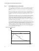
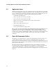
Systems may be characterized by their failure intensity over time. Generally, newly deployed

systems exhibit higher failure rates with defect removal occurring over the near term as a system is

deployed into new environments. These residual design faults are common in new systems. Their

removal is a trend of decreasing failure intensity. Eventually, systems generally achieve a

stabilization of reliability over time when changes to the system and environment are no longer

common. The failure intensity increases as changes to the system or environment happen (e.g., new

versions of hardware and/or software are added to the system). Over time, the unavailability (A)

curve looks something like Figure 7 [Lapr92]:

Figure 7. Unavailability Curves

A(t)