Quick Start Guide

32 Quick Start Guide
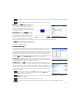
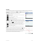
1. Tap the cell with the HP logo in it (at the top left corner). Alternatively, you can use
the cursor keys to move to that cell (just as you can to select a column or row
heading).
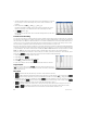
2. On the entry line type S.RowfnCol+1
Row and Col are built-in variables. They represent the row number and column
number, respectively, of the cell that has a formula containing those values.
3. Tap or Press E.
Each column gives the nth power of the row number starting with the squares. Thus
9
5
is 59,049.
Cell references and naming
You can refer to the value of a cell in formulas as if it were a variable. A cell is referenced by its column and row coordinates,
and references can be absolute or relative. An absolute reference is written as $C$R (where C is the column number and R
the row number). Thus $B$7 is an absolute reference. In a formula it will always refer to the data in cell B7 wherever that
formula, or a copy of it, is placed. On the other hand, B7 is a relative reference. It is based on the relative position of cells.
Thus a formula in, say, B8 that references B7 will reference C7 instead of B7 if it is copied to C8.
Ranges of cells can also be specified, as in C6:E12, as can entire columns (E:E) or entire rows ($3:$5). Note that the alphabetic
component of column names can be uppercase or lowercase except for columns g, l, m, and z. These must be in lowercase
if not preceded by $. Thus cell B1 can be referred to as B1,b1,$B$1 or $b$1 whereas M1 can only be referred to as m1,
$m$1, or $M$1. (G, L, M, and Z are names reserved for graphic objects, lists, matrices, and complex numbers.)
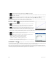
Cells, rows, and columns can be named. To name a cell, row, or column, go the cell, row header, or column header, enter a
name and tap . The name can then be used in a formula. Consider the following example:
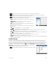
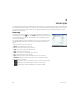
1. Select cell A (that is, the header cell for column A).
2. Enter COST and tap .
3. Select cell B (that is, the header cell for column B).
4. Enter S.COST*0.33 and tap .
5. Enter some values in column A and observe the calculated results in column B.
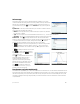
Copy and paste
Select one or more cells and press SV. Move to the desired location and press
(M). You can choose to paste either the values, formulas, or formats (or the formula
and associated format).
Menu items
• —Activates the entry line, where you can enter or edit whatever is selected.
• —Names whatever is selected. This item appears only when you start entering content or after you tap .
• —Forces what you are about to enter to be evaluated by the CAS. For example, S.23t2 yields 11.5
normally, but if you precede the calculation by tapping , the result displayed is 23/2. You can revert to non-CAS
evaluation by tapping . These menu items appear only when you start entering content or after tapping .
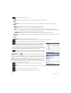
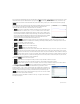
• —Displays an input form, where you can specify the cell you want to jump to.
• —Sets the calculator into select mode so that you can easily select a block of cells using the cursor keys. It
changes to to enable you to deselect cells. (You can also press, hold, and drag to select a block of cells.)
• or —Sets the direction the cursor moves after content has been entered in a cell.