OWNER’S MANUAL MicroTSCM Streaming Current Monitor HF scientific 3170 Metro Parkway Ft. Myers, FL 33916 Phone: 239-337-2116 Fax: 239-332-7643 EMail:HFinfo@Watts.com Website: www.hfscientific.com 21648 (07/09) REV 2.
Table of Contents Section Page Specifications ................................................................................................... 1 1.0 Overview........................................................................................................... 2 1.1 Unpacking and Inspection of the Instrument and Accessories .................... 2 2.0 Safety ................................................................................................................ 2 2.
Table of Contents (continued) Section Page 8.0 Additional Features and Options ................................................................ 18 8.1 Sensor Gain Switch ............................................................................. 18 8.2 Remote Panel Meter ............................................................................ 18 8.3 Optional Flow Switch.......................................................................... 18 9.0 Routine Maintenance ...........................
Specifications Measurement Range ± 10.0 SCU or ICu Accuracy ± 1 % of Full Scale Repeatability 1% Linearity ± 1% Resolution 0.01 SCU or ICu Response Time 1 second Analyzer Display Backlit Graphical LCD with trending Alarms Two Programmable, One Sensor, 120-240VAC 2A Form C Relay Analog Output Powered 4-20 mA, 1000 Ω drive Communications Port Optional RS-232 or RS-485 Flow Rate 6.0 – 9.5.0 L/min. (1.5 -2.
1.0 Overview The SCM–Streaming Current Monitor allows for optimizing and control of dosing coagulants used for clarification of water. Although the analyzer is capable of displaying the units in either SCU’s or ICu, this manual will always refer to SCU. 1.1 Unpacking and Inspection of the Instrument and Accessories The table below indicates the items in the shipment.
3.0 Theory of Operation In a liquid form, water molecules move around each other at a fast rate. One affect of this fast movement is the ability to suspend matter. This phenomenon is called “Brownian Motion”. It occurs when microscopic particles are maintained dispersed in suspension due to their random bombardment by the fast movement of water molecules. Typical particles found in raw water entering WTP have finely divided clay particles and organic matter collectively called silt.
Additive Chemicals + + + - + - + - + - - + + - + + - + - + + + - + + + + - + - - - + + + + - + + + + Contaminant Particles - - - + + - + - + + + - - + + - - - - - - + - + + + + + - - + + - - + + + + + 1. Charge Neutralization 2. Bridging Figure 1: Effects of Chemicals 3.1 Treatment of Water for Clarification Most water treatment chemicals consist of a cationic (positively charged) chemical e.g.
TURBIDITY CHEMICAL DOSAGE ppm Figure 3: Turbidity vs Dosage 3.2 Charge Analysis Charge analysis is the measurement of the electro kinetic charge of a solution due to the presence of charged particles. The electro kinetic charge can be measured by a number of different methods. 1. Applied electric field Measurement: The relative mobility of the solid or liquid phase. This is the first method developed for calculating the Zeta Potential.
4.0 Installation and Commissioning 4.1 Sample Point Careful consideration must be given to where in the system the sample will be taken. Streaming current monitoring requires sampling of the raw water after the introduction of coagulant. It is critical that that the sample point is far enough from the dosage point to ensure good mixing. The sample point should be at least 10 pipe diameters away from the dosing point to ensure ample mixing.
4.3 Sensor Mounting & Plumbing Locate the sensor as close to the sampling point as possible to reduce lag time. A site that is protected from the elements (sun, rain etc.) is preferred, but the sensor is rated for use under most outdoor conditions. The sample chamber is designed to be mounted with ¼” diameter bolts. The sensor does not get firmly mounted, but just sits on top of the sample pot. A light shield protects the clear sample pot cover & helps to prevent algae growth.
4.4 Analyzer Mounting The analyzer is not weather tight and this must be taken into consideration during site selection. The analyzer provides the control outputs via 4-20 mA and alarms. It is recommended that the analyzers be mounted in a location for easy viewing and keypad access. The analyzer can be flipped on its mount to gain access to the electrical connections. Please refer to the drawing below for mounting dimensions and hole location. Figure 5: Analyzer Mounting MICROTSCM (07/09) REV 2.
4.5 Electrical Connections All of the electrical connections to the instrument are made at the termination area which is located in the back of the analyzer under the access cover. Refer to Figure 6 carefully as the wire colors do not follow the actual PCB screen printing. For easy access, loosen the two clamping knobs and rotate the instrument upside down. Remove the access cover. Figure 6: Analyzer Electrical Connections 4.5.
Terminal J6 Connection Purpose Impedance Terminal 1 0-10V 50K ohm or greater Terminal 2 0-1V 5K ohm or greater Terminal 3 0-100 mV 500 ohms or greater Terminal 4 Common N/A The 4-20 mA connection is made at J5. Terminal 1 is positive, Terminal 2 is negative. The recorder load may be up to 1000 ohms. Galvanic isolation may be achieved by removing the jumper at J13. This procedure will require the removal of the entire rear cover assembly. 4.5.
5.0 Operation The SCM system consists of three major components, The Sensor, the Sample Chamber and the Analyzer. 5.1 The Sensor/Sample Chamber The sensor module sits on top of the sample chamber, with the probe end below the water level. The sample chamber has three valves to adjust the flow: • The inlet should be adjusted such that there is always a sample present. A lack of a sample will cause premature wear in the cell and piston.
5.3 The Graphing Screen Shown below in Figurer 7 is the main graphing screen. The numbers are used to identify various features. 1. The larger number area shows the current reading and units used. 2. The graph time base. Options are 8 or 24 hours and can be set in the Display Parameters Menu. 3 & 4. The upper and lower display limits. These are settable in the Display Parameters Menu. Please note that these settings also affect the 4-20 mA /Voltage range. 5 & 6. Alarms 1&2.
5.4 Menus The following flow chart can be referred to for the menu structure. Figure 8: Menu Flow Chart MICROTSCM (07/09) REV 2.
6.0 Calibration The MicroTSCM has been calibrated at the factory, however to ensure accuracy it is recommended that the instrument be calibrated prior to being placed online. Long term drift may occur in this instrument and HF scientific recommends calibration every three months. To facilitate the initial calibration, a calibration kit, Part # 19922 is supplied with this instrument. When prepared according to the included instructions a +5.30 SCU Cationic calibration solution is produced.
7.0 Automatic Control This section describes the use of the SCM to control the process. It is recommended that a review of section 4.1 (sample point) is made to ensure correct installation. 7.1 Optimization of Treatment Process Prior to turning control over to the SCM, it is crucial to optimize coagulant dosing. The optimum point is obtained when the minimum coagulant can be fed that produces the desired results for any particular treatment process. This should be done slowly and in steps.
given change in coagulant dosing. The Integral Time tells the instrument how long it will take to fully realize the effects of a change in coagulant dosing. 7.3 PI Control Procedure The assumption is that the wiring between the MicroTSCM analyzer and the dosing pump has been installed. The following procedure is recommended to determine the correct Proportional - Integral (PI) values for any particular system. The MicroTSCM analyzer is used to slow down the control loop to prevent overdosing of coagulant.
Convert the effected change in SCU to a percentage. Since the instrument always operates in a range of +10 SCU to -10 SCU, the range is 20 SCU. X Effect Range Then calculate the proportion band or PB. % effect = PB = % Effect % Cause X 100 1 100 1 In our example calculating the Proportional Band or P. Band with a 10% change (cause): % effect = 0.5 SCU 20.0 SCU X 100 1 = 2.5% X 100 = 25% PB = 2.5% 10% 1 To prevent overshoot, it is desirable to slow the control loop down a little more.
8.0 Additional Features and Options 8.1 Sensor Gain Switch The gain toggle switch is mounted on the side of the sensor housing. The purpose of the gain switch is to increase the magnitude of the sensor’s response. The gain switch can be used in applications where little response is noted to changes in coagulant dosing. When deciding to use the gain switch try the LOW setting first. If the response is not adequate, use the HIGH setting.
9.0 Routine Maintenance The most important maintenance procedure is to keep the sensor clean. The need for cleaning is indicated when normal readings cannot be maintained. As a preventative measure, cleaning intervals of 30 days or less is recommended. There are two recommended cleaning methods. 9.1 Preferred Method – Chemical Cleaning Pour the SCM-1 cleaning solution (Catalog # 19402) into a suitable container, large enough to immerse the lower 1/2 of the probe body.
Figure 10: Sensor – Exploded View 9.3 Analyzer Fuse The analyzer fuse located in a cartridge on the cord receptacle in the back of the instrument. To gain access, remove the four access cover screws and remove the power cord. Insert a screwdriver into the slot and pry to remove the cartridge. Be certain to match the desired voltage with the indication arrow when reinserting the cartridge. Figure 11: Fuse MICROTSCM (07/09) REV 2.
10.0 Troubleshooting 10.1 Diagnostic Chart Symptom Solutions Analyzer Display Not Lit. 1. Make sure the unit is plugged in and turned on. 2. Make certain that the power source is providing the correct voltage. 3. Make sure the analyzer is set for the correct voltage. 4. Check analyzer fuse. Sensor probe not moving 1. Check the interconnect cable connection at the sensor. 2. Check the wiring of the interconnect cable on the back of the analyzer and inside the sensor. 3.
11.0 Accessories and Replacement Parts List The items shown below are recommended accessories and replacement parts. Accessory Catalog Number Cleaning and Descaling Solution 19402 Optical Isolated RS-485 Interface Kit 20519 RS-232 Interface Kit 19861 Flow Alarm 19886 Calibration Kit 19922 Interconnect Cable 7.6 meter (25 Ft.) 22480 Operating & Maintenance Manual 21648 To order any accessory or replacement part, please contact the HF scientific Customer Service Department.
12.0 Definitions Anionic: Negative charged ions. Automatic Control: Placing the control of the dosing pumps under the control of the Streaming current monitor. The Optional PI controller is recommended. Brownian Motion: A phenomenon which occurs when microscopic particles are suspended in a solution due to their random bombardment by the fast movement of water molecules. Cationic: Positive charged ions. ICu: Ion Charge unit. 1 ICu is approximately equal to 1 mA of charge. 1 ICu = 1 SCU.
13.0 Warranty HF scientific, as vendor, warrants to the original purchaser of this instrument that it will be free of defects in material and workmanship, in normal use and service, for a period of one year from date of delivery to the original purchaser. HF scientific’s, obligation under this warranty is limited to replacing, at its factory, the instrument or any part thereof.
HF scientific Installation Evaluation Use this worksheet to help establish a baseline for optimal dosing. Readings every 6 hours are recommended.