Reference Manual

3−3
applied and elevation changes have been
neglected (again using upstream conditions as a
reference):
òV
1

2
2g
c
) P
1
+
òV
VC

2
2g
c
) P
VC
 ( 6 )
In the equation below, equation 5 has been
inserted and rearranged:
P
VC
+ P
1
*
òV
1

2
2g
c
ƪ
ǒ
A
1
A
VC
Ǔ
2
* 1
ƫ
(7)
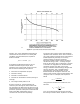
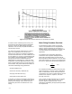
Thus, at the point of minimum cross sectional
area, we see that fluid velocity is at a maximum
(from equation 5 above) and fluid pressure is at a
minimum (from equation 6 above).
The process from the vena contracta point to a
point several diameters downstream is not ideal,
and equation 2 no longer applies. By arguments
similar to the above, it can be reasoned (from the
continuity equation) that, as the original cross
sectional area is restored, the original velocity is
also restored. Because of the non-idealities of this
process, however, the total mechanical energy is
not restored. A portion of it is converted into heat
that is either absorbed by the fluid itself, or
dissipated to the environment.
Let us consider equation 1 applied from several
diameters upstream of the restriction to several
diameters downstream of the restriction:
U
1
)
V
1

2
2g
c
)
P
1
ò
)
gZ
1
g
C
) q +
U
2
)
V
2

2
2g
c
)
P
2
ò
)
gZ
2
g
C
) w
(8)
No work is done across the restriction, thus the
work term drops out. The elevation changes are
negligible and as a result, the respective terms
cancel each other. We can combine the thermal
terms into a single term, H
I
:
òV
1

2
2g
c
) P
1
+
òV
2

2
2g
c
) P
2
) H
I
 ( 9 )
The velocity was restored to its original value so
that equation 9 reduces to:
P
1
+ P
2
) H
I
(10)
Consequently, the pressure decreases across the
restriction, and the thermal terms (internal energy
and heat lost to the surroundings) increase.
Losses of this type are generally proportional to
the square of the velocity (references one and
two), so it is convenient to represent them by the
following equation:
H
I
+ K
I

òV
2
2
 (11)
In this equation, the constant of proportionality, K
I
,
is called the available head loss coefficient, and is
determined by experiment.
From equations 10 and 11, it can be seen that the
velocity (at location two) is proportional to the
square root of the pressure drop. Volume flow rate
can be determined knowing the velocity and
corresponding area at any given point so that:
Q + V
2
A
2

2(P
1
* P
2
)
òK
I
Ǹ
A
2
(12)
Now, letting:
ò + Gò
W
and, defining:
C
V
+ A
2

2
ò
W
K
I
Ǹ
 (13)
Where G is the liquid specific gravity, equation 12
may be rewritten as:
Q + C
V

P
1
* P
2
G
Ǹ
 (14)
Equation 14 constitutes the basic sizing equation
used by the control valve industry, and provides a
measure of flow in gallons per minute (GPM)
when pressure in pounds per square inch (PSI) is
used. At times, it may be desirable to work with
other units of flow or independent flow variables
(pressure, density, etc). The equation
fundamentals are the same for such cases, and
only constants are different.
Determination of Flow Coefficients
Rather than experimentally measure K
I
and
calculate C
v
, it is more straightforward to measure
C
v
directly.