User's Manual

HARSFEN0602
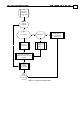
The user provides, for each motion interval, the boundary positions and speeds. Mathematically, the user
provides the following data:
The starting position and speed, denoted by P0 and V0, respectively
The end position and speed, denoted by PT and VT, respectively.
Let
0
t denote the starting time, and let T denote the length of the time interval.
The position for
]Tt,t[t
00
+∈ is given by the 3
rd
order interpolating polynomial:
d)tt(c)tt(b)tt(a)t(P
0
2
0
3
0
+−+−+−=
The speed is given by:
c)tt(b2)tt(a3)t(V
0
2
0
+−+−=
The four parameters a, b, c, and d are unknown. They can be solved using the four linear equations
0P)t(P
0
= , Namely 0Pd .
0V)t(V
0
= , Namely 0Vc
PT)Tt(P
0
=+ , Namely dcTbTaTPT
23
+++=
VT)Tt(V
0
=+ , Namely cbT2aT3VT
2
++=
Example
In this example, we demonstrate how very few points can accurately describe a smooth and long motion
path.
Consider two Amplifiers, driven synchronously do draw an ellipse. One Amplifier drives the x-axis, and the
other drives the y-axis.
The long axis of the ellipse is 100000 counts long, and the short axis of the ellipse is 50000 counts long. The
entire ellipse is to be traveled within 2.2 seconds.
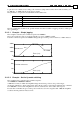
We planned a PVT motion with a fixed inter-point time of 100millisec. 23 points are enough for the entire
ellipse, as seen in the figures below. The motion is planned so that the tangential speed is accelerated to a
constant rate, and then decelerated back to zero speed at the end of the ellipse. Near the starting point of the
ellipse, the speed is slow – and therefore the PVT points, which are equally spaced in time, are more
spatially dense there. The continuous line in the figure below depicts the true ellipse and also the ellipse
generated by the Amplifier by interpolating the PVT points.
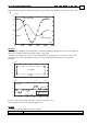
The original ellipse and the Amplifier interpolation of the PVT points are so close, that they can't be resolved
on the plot.