• Internal Temp: Indicates the current internal temperature of the M.O.L.E. Profiler. • RF Status: Signal strength indicator with 5 bars indicating relative strength of the RF signal. Save: • Stops the M.O.L.E. Profiler logging real-time data and allows the user to save that data. If there is not enough data recorded, the software displays a “Not enough data to profile” message, and it will cancel the data run. When real-time data is logging using the MEGAM.O.L.E.® or SuperM.O.L.E.
When real-time data logging has stopped, the software automatically processes the data. Depending on how long the data run is, it may take a few moments to complete. 7) Click the Save command to save the data run. The software prompts the user to specify a file name (*.XMG). When saving a data run (*.XMG) to a different file directory other than the current Working directory, the software automatically sets the new file directory as the current Working Directory.
8) When finished, click the Save command button to complete the process. When using the PTP® VP-8, the PTP® TX power must be turned OFF after saving the data run by removing the On/Off Male Plug connector from the Female On/Off Power connector. Wireless RF communication tips (MEGAM.O.L.E.® & SuperM.O.L.E.® Gold 2): RF signals come and go as either the M.O.L.E. Profiler moves through the oven or the Transceiver is moved around like FM radio static as you drive in your car.
The transmitting Antenna and its proximity to metal can have a big affect. Care should be taken to make sure the Antenna is not laying on metal parts in the machine or barrier box. Keeping the Antenna straight is best. Wireless RF Range 5.5.5.4. Set Recording Parameters The Set Recording Parameters command configures how the M.O.L.E. profiler records data during a data run. This is available when in Engineer Mode.
To set recording parameters: 1) Connect the M.O.L.E. Profiler to the computer. Refer to Basics>Setup>Communications Setup for more information. If an instrument is not currently connected to the computer, the default Demonstration MEGAM.O.L.E.® profiler will be displayed. 2) On the M.O.L.E. menu, click Set Recording Parameters. The Start and Stop Parameters are optional settings and do not require configuration. 3) In the Instrument Name text box, type a company, operator, or M.O.L.E. Profiler name.
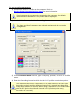
5) If desired, configure a Start Parameter such as a threshold temperature or Delay Points by selecting the associated check box and entering the proper values. Specifying a threshold temperature “triggers” the recording process when any active channel reaches the specified temperature and Data Points “trigger” the M.O.L.E. profiler to start recording when the specified data point is reached in the process. The actual delay is equal to the Interval times the Pts Dly.
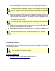
When navigating through the wizard, the step list on the left uses a color key to inform the user of the current step, steps that have been completed and remaining steps. Current Completed Remaining 3) Select the desired instrument from the dialog box. If there is none displayed, select the Scan for Instruments command button to detect all connected instruments. If the software does not detect a M.O.L.E.
) Select the Next command button to send the data listed in the dialog box to the instrument. If the currently selected M.O.L.E. Profiler is a SuperM.O.L.E. Gold, the sending of data will erase the data currently stored in the M.O.L.E. Profiler. 9) Verify the instrument status. This dialog box displays the health of the M.O.L.E. Profiler such as battery charge, internal temperature, thermocouple temperatures.
10) Select the Finish command button to complete the Setup Instrument wizard. 5.5.5.6. Show on Profile M.O.L.E. status information can be displayed or hidden on the Data Graph. This is available when in Engineer Mode. To show machine information on the Data Graph: 1) On the M.O.L.E. menu, click Show on Profile. 2) Select or clear the associated machine characteristics to display or hide on the Data Graph.
3) Click the OK command button to accept, or Cancel to quit the command. 5.5.6. Machine-Oven Menu The Machine-Oven menu include options to design specific machine models. Creating an machine model allows the user to visualize it on the Data Graph along with the associated data run profile.
5.5.6.1. Set Machine Information This command allows the user to set machine information and display it on the Data Graph so the user can visually see how the data run profile lines up with the machine. This is available when in Engineer Mode. To set machine information: When setting machine information, this data will be applied to the currently selected data run only. Existing defined machine models may not accurately reflect your machine and are used as a starting template.
2) Select your machine from the Machine drop down list. If it does not appear in the list click the New command button to create a new one. Refer to topic Software>Menus>Machine>Create new Machine for more information. 3) Set the machine conveyor speed. The software uses this value to calculate the Time (X) Scale values when Distance units are displayed. This number is also used as the actual conveyor speed when prediction data lines are added.
5) Set the Zone Temperatures in the zone matrix. These temperatures could be the upper and lower thresholds of acceptable temperatures to meet process standards or temperature settings of upper and lower heat sources. Upper zone temperatures appear as solid lines and lower zones appear as dotted lines on the Data Graph. 6) Click the OK command button to set the machine information, or Cancel to quit the command.
To view machine information: 1) On the Machine-Oven menu, click View Machine Information. 2) Select the Cancel command button to quit the command. 5.5.6.3. Create New Machine When setting machine information, the user is required to select a machine. The software includes basic machine models for the user to select from. If your machine model does not appear in the list the software has the ability for you to create a new machine model. This is available when in Engineer Mode.
3) Enter the amount of heating and cooling zones. As zones are specified the zone matrix will automatically grow to allow you to enter zone measurements. 4) Select the assembly flow (left to right or right to left), zone measurement method (individual or accumulative) and units of measurement. Refer to the illustration below for proper measurement methods.
5) Enter the zone measurements in the zone matrix. 6-) Click the Save command button to save the new machine, or Cancel to quit the command. The new machine will now appear in the Machine drop-down list on the Set Machine Information dialog box. Refer to topic Software>Menus>Machine>Set Machine Information for more information.
5.5.6.4. Adjust Zones This command allows the user to manually adjust the displayed machine zones on the Data Graph. To use this command a machine must be selected and displayed. Refer to topic Software>Menus>Machine>Set Machine Information. This is available in both Engineer & Verify Modes. To adjust zones: 1) One the Machine-Oven menu, click Adjust Zones to activate. A check mark appears to the left of the command indicating the software is in Adjust Zones mode.
5.5.6.5. Estimate Conveyor Speed To properly display a machine model on the Data Graph, a conveyor speed must be set. If you do not know what the conveyor speed is when setting machine information, the software allows you to estimate it based on the machine information and the data run profile. This is available when in Engineer Mode. To estimate conveyor speed: 1) On the Machine-Oven menu, click Estimate Conveyor Speed. and the estimated conveyor speed automatically is displayed in the text box.
3) Click the OK command button to accept, or Cancel to quit the command. 5.5.7. Assembly-Board Menu The Assembly-Board menu include commands that enable the user to set and edit experimental assembly documentation.
5.5.7.1. Set Assembly Information This command allows the user to set assembly information associated with the selected data run profile. This is available when in Engineer Mode. To enter assembly information: When setting assembly information, this data will be applied to the currently selected data run only. 1) On the Assembly-Board menu, click Set Assembly Information. If a setting is already selected for a data run, the software prompts the user to decide if they wish to modify the current data run.
2) Enter an assembly part number. 3) Click the Notes command button if you would like to enter part documentation about the test assembly being profiled.
4) Click the image file Browse command button to select a product image. Image files supported by the software are Jpeg (.jpg), Bitmap (.bmp), and Tiff (.tif). 5) Enter the test assembly board length, width and thickness. 6) Enter the sensor location descriptions. These descriptions can be the location where each sensor is connected to the test product. The channel color associated with the description indicates which Data Plot on the Data Graph it represents.
Thermocouple placement information entered in the sensor location matrix are also displayed as the Sensor Locations in the Data Table. 7) Enter sensor location dimensions. Sensor Locations can also be set by dragging sensor location markers on the selected image. To move the markers, click the Enlarge command button below the assembly image and the Set Sensor Locations dialog box appears. Specified X-dimensions may be altered when using the Align Profile Peaks command to align the data run profile lines.
9) Click the OK command button accept or Cancel to quit the command. 5.5.7.2. View Assembly Information This command allows the user to view assembly information associated with the selected data run profile. This is available when in Verify Mode. To view assembly information: 1) On the Assembly-Board menu, click View Assembly Information.
2) For a larger view of the assembly image and sensor locations, click the Enlarge command and the View Sensor Locations dialog box appears. 3) Select the OK or Cancel command button to close the dialog box.
4) Select the Cancel command button to quit the command. 5.5.7.3. Show on Profile Assembly name can be displayed or hidden on the MAP data section of the Data Graph. This is available when in Engineer Mode. To show assembly information on the Data Graph: 1) On the Assembly-Board menu, click Show on Profile. 2) Select or clear the Assembly name check box to display or hide it on the Data Graph. 3) Click the OK command button to accept, or Cancel to quit the command. 5.5.8.
5.5.8.1. Set Process Information This command allows the user to set a process paste and display it on the Data Graph so the user can visually see how the data run profile lines up with the process specification. This is available when in Engineer Mode. To set a process: When setting a process, this data will be applied to the currently selected data run only. Existing defined machine models may not accurately reflect your machine and are used as a starting template.
2) Select your process specification. Select a Paste from the database or previously created Target 10 Specification. If your Paste does not appear in the database list click the New command button to create a new one. Refer to topic Software>Menus>Process>Create new Paste for more information. When the user selects a paste from the database, they can use the radio buttons below the drop down box to filter and display only the user created pastes from paste database.
4) Click the Notes command button if you would like to enter process paste documentation. 5) Click the OK command button to set the process, or Cancel to quit the command. To view the process on the Data Graph, the Show on Profile settings must be enabled. Refer to topic Software>Menus>Process>Show on Profile for more information.
5.5.8.2. View Process This command allows the user to view process information associated with the selected data run profile. This is available when in Verify Mode. To view a process: 1) On the Process-Paste menu, click View Process. 2) Select the Cancel command button to quit the command. 5.5.8.3. Create New Paste When setting machine information, the user is required to select a machine. The software includes basic machine models for the user to select from.
This is available when in Engineer Mode. To create a new paste: 1) On the Process-Paste menu, click Create New Paste. 2) Enter the required information and select the Next button. 3) Enter the RAMP – Slope information and select the Next button. 4) Enter the SOAK –Temperatures information and select the Next button.
5) Enter the SOAK –Time information and select the Next button. 6) Enter the SPIKE – Ramp Slope information and select the Next button.
7) Enter the SPIKE – Time Above information and select the Next button. 8) Enter the SPIKE – Peak Temperature information and select the Next button.
9) Enter the SPIKE – Cooling Slope information and select the Finish button to create the new paste and return to the Paste Specification database dialog box. Once the user proceeds to each Step, the Back button can be selected to confirm or modify previously entered information. 10) Click the Finish command button to accept, or Cancel to quit the command. The new process paste will now appear in the Paste drop-down list on the Set Paste dialog box.
5.5.8.4. Show on Profile Process Paste specification can be displayed or hidden on the Data Graph. This is available when in Engineer Mode. To show the process paste specification on the Data Graph: 1) On the Process-Paste menu, click Show on Profile. 2) Select or clear the associated process paste options to display or hide on the Data Graph. 3) Click the OK command button to accept, or Cancel to quit the command. 5.5.9.
5.5.9.1. Set Temperature (Y) Scale This command controls the scale of the Temperature (Y) axis on the Data Graph. This is available in both Engineer & Verify Modes. To use the scaling command: 1) On the Profile menu, click Set Temperature (Y) Scale. This dialog box identifies the current settings of the displayed units and the maximum and minimum values. 2) Select between Auto or Manual mode.
temperature settings are visible in the Data Graph. In Manual mode, the range of values must be manually set. 3) Click the OK command button to use the settings or Cancel to quit the command. The software allows the ability to include recipe values when using the Autoscale feature. Instead of automatically scaling the Data Graph to the data run profile, it scales it to include the recipe values along with profile so the data will always be visible and easy to work with.
3) Select the line color by clicking the line button below the label. When an reference line is displayed on the Data Graph, the default label is the specified temperature. The software allows the user to rename the line by using the Optional Name text box. 4) Click the OK command to accept the new settings or Cancel to quit the command. This command can also be accessed by right-clicking the scale on the Data Graph and select Add Temperature (Y) Scale from the shortcut menu.
To move an Temperature (Y) Reference Line: 1) Position the mouse pointer over the desired reference line. 2) Double-click the reference line and the Add Temperature (Y) Reference line dialog box appears. 3) Edit the reference line settings and click the OK command to accept the new settings or Cancel to quit the command. 5.5.9.3. Set Time (X) Scale This command controls the scale of the Time (X) axis on the Data Graph. This is available when in Engineer Mode.
Points Scale Absolute Time Scale This command can also be accessed by right-clicking the scale on the Data Graph and select Set Time (X) Scale from the shortcut menu. 5.5.9.4. Add Time (X) Reference Lines Time Reference Lines are colored vertical lines that can be positioned anywhere within the range of X-values on the Data Graph. These reference lines indicate the temperature values at the intersection of a Data Plot with each displayed reference line. This is available when in Engineer Mode.
When a reference line is displayed on the Data Graph, the default label is the next number of reference line. For example if there is two reference lines displayed, the next default label will be 3. The software allows the user to rename the line by using the Name text box. 3) Click the OK command to accept the new settings or Cancel to quit the command. If a reference line is used in a Data Table calculation, the name of the reference appears in the header along with the parameter value.
When moving the selected Time (X) Reference line, it can be moved past other cursors to any location on the Data Graph. When a Time (X) Reference line is moved to a new position, it snaps to the closest real Time (X) value. Notice on highly magnified graphs that the line jumps from point to point. The values in the Data Table are automatically updated to reflect the new position. 5.5.9.5.
When downloading a data run from the M.O.L.E. Profiler, the default sensor alignment can be specified in the Profile tab of the Preferences dialog box. Refer to topic Software>Menus>File>Preferences>Profile for more information. 5.5.9.6. Align Profile to Dimensions If sensors are placed so they enter and exit machine zones at different times, the resulting Data Plots lag behind one another.
A conveyor speed and sensor locations must be set to properly use this command. Refer to topic Software>Menus>Machine>Set Machine Information and/or Software>Page Tabs>Profile>Data Graph>Conveyor Speed Indicator for more details. 1) On the Profile menu, click Align Profile To Dimensions the channel lag values are automatically calculated, and the Data Plots adjust to reflect them. A check mark appears to the left of the command indicating the software is in Align Profile To Dimensions mode.
This is available when in Engineer Mode. To show profile information on the Data Graph: 1) On the Profile menu, click Show on Profile. 2) Select or clear the File Name check box to display or hide it on the Data Graph. 3) Click the OK command button to accept, or Cancel to quit the command. 5.5.10. Tools Menu Options in this menu help the user manipulate and analyze the data run profile displayed on the Data Graph.
5.5.10.1. Magnify The Magnify tool enlarges any selected area of the data graph for easy visual examination. This is available when in Engineer Mode. To magnify a portion of the Data Graph: When a Magnified Window constraint is applied to a parameter in the Data Table, the Magnify tool is used to enlarge a portion of the Data Graph, and the values within the magnified area are displayed in the Data Table. 1) On the Tools menu, point to Magnify then select Select Area.
4) Release the left mouse button when the outline of the area to be magnified is visible. The area inside the box is then magnified to fill the entire Data Graph.
To show even more detail in the Data Graph, Magnify can be performed multiple times. If the Magnify tool reaches the maximum zoom capability the software will display a message box informing that the user has “Zoomed to Tight”. This command can be accessed on the Toolbar when the Profile Tab is active. Magnify Button 5.5.10.2. Slope The Slope tool finds the average slope between any two points in the Data Graph. This is available when in Engineer Mode.
2) 3) 4) 5) Position the mouse pointer at a point on the curve. Press and hold the left mouse button. Drag the pointer to the end of the desired slope line. Release the left mouse button when the pointer is at the desired location. The software will draw a slope line on the Data Graph, and label the slope value. To obtain more accurate slopes: 1) On the Tools menu, click Magnify to magnify a portion of the Data Graph 2) Repeat the Slope command.
To remove a slope line from the Data Graph: 1) Using the mouse pointer, select the object on the Data Graph by clicking it once. The object trackers will then become bold indicating that it has been selected. 2) Press the [Delete] key on the keyboard to remove the object.
Slope Applications • Use the Slope tool to find the average slope between any two points on the graph. Longer slope lines tend to produce more accurate slope calculations. • The Slope tool can be used to compare actual data with ideal conditions by drawing a line with a known slope (to represent the ideal condition) beside a portion of a Data Plot. Slope Limitations • Slope calculations are based on logged points connected by the slope line.
5.5.10.3. Peak Difference This command displays the difference in value between the peak of the maximum Data Plot and the peak of the minimum Data Plot in any location of the Data Graph. This command is especially useful for measuring side-to-side heating differences in a machine (oven). This is available when in Engineer Mode. To display the peak difference between Data Plots: The peak difference is calculated as the maximum difference between the highest peak and the lowest peak within the rectangle.
1) Using the mouse pointer, select the object on the Data Graph by clicking it once. The object trackers will then become bold indicating that it has been selected. 2) Press the [Delete] key on the keyboard to remove the object. This command can be accessed on the Toolbar when the Profile Tab is active. Peak Difference Button 5.5.10.4. Overlay The Overlay tool displays a second data run profile over the currently displayed profile on the Data Graph for comparison. This is available when in Engineer Mode.
2) Select a data run file (.XMG) to overlay on the original. The profile will be inserted at the same process origin and automatically scaled to the same Temperature (Y) axis. The original Data plots remain as solid lines while those added for comparison are dashed. The dashed “Overlay” Data Plots are the same color as the original Data Plots. To remove the overlaid Data Graph: 1) Select the Overlay command again.
must be done to the overlaid data run file prior to using the Overlay tool. Save that data run file and use the Overlay tool again. This command can be accessed on the Toolbar when the Profile Tab is active. Overlay Button 5.5.10.5. Measure The Measure tool is similar to the Slope tool except it measures the distance between any two points on the Profile worksheet Data Graph.
To obtain more accurate distances: 1) Magnify a portion of the Data Graph using the Magnify tool and repeat this procedure. To remove the annotated distance: 1) Using the mouse pointer, select the object on the Data Graph by clicking it once. The object trackers will then become bold indicating that it has been selected. 2) Press the [Delete] key on the keyboard to remove the object.
This command can be accessed on the Toolbar when the Profile Tab is active. Measure Button 5.5.10.6. Notes The Notes tool adds a leader with text to any portion on the Data Graph to label special points of interest. This is available in both Engineer & Verify Modes. To add notes to the Data Graph: 1) On the Tools menu, click Notes.
3) A dialog box appears allowing the user to enter a note by typing it in the text box. There also are options to customize the color and font size. 4) Click the OK command button or Cancel to quit the command. To move notes: 1) Select a note leader, click and drag the mouse pointer to the desired location for the note and release the mouse button. To remove notes: 1) Using the mouse pointer, select the object on the Data Graph by clicking it once.
This command can be accessed on the Toolbar when the Profile Tab is active.
5.5.10.7. Crop The Crop tool allows the user to save a portion of the data run profile that eliminates unwanted portions from it. This crop tool only works for the Time (X) Scale which allows the user the ability to remove portions from the front and back of the data run profile. This is available when in Engineer Mode. To crop a data run profile: 1) On the Tools menu, click Crop. 2) Position the mouse pointer on any area of the Data Graph you want to start the crop.
When saving a cropped data run file, the software allows the user to save as the existing file name or give it a different one. This helps preserve the original data run. Once the cropped data run has been saved, it Autoscales to properly appear in the Data Graph.
5.5.10.8. Prediction One of the most impressive software features is the Prediction tool. This tool enables the user to change a zone temperature value or the conveyor speed and predict the outcome of that change. Prediction is easy to use and a valuable command that quickly defines process parameters. To use the Prediction Tool machine information must first be set to build an accurate “model” of an machine (oven) environment.
If sensor temperatures are inconsistent with zone temperature settings, a message box with an explanation appears. The explanation appears only once for all zones, each time Prediction is used. After that, the software assumes the user is aware of the potential problem. The inconsistent setting does not prevent the software from making a prediction. It makes a rational assumption about what is happening.
2) Experiment by making “what if” changes to the conveyor speed and sliding Zone Temperature Prediction Handles up or down to the preferred prediction temperature. If the Top and Bottom zone temperature setpoints are different, the software allows the user to perform predictions by adjusting them independently. Refer to topic Set Machine Information.
3) Once the predicted machine recipe is at the desired settings, the user can save them to a recipe file (.XMR) or print them by selecting the Save Recipe command button.
4) Once the machine recipe is saved, set the machine to the final prediction values, let it stabilize and then perform another data run to check if the process has been optimized. This command can be accessed on the Toolbar when the Profile Page Tab is active. Prediction Button 5.5.11. Help Menu The Help menu commands are useful when information is needed quickly or when this Users guide is not available.
5.5.11.1. Help The Help Index is a complete reference tool that can be used at any time. This is available in both Engineer & Verify Modes. To launch the help system: 1) On the Help menu, click Help to launch the user’s help guide. You may now search for the help topic of your choice.
This command can be accessed on the Toolbar and can also be used by pressing the shortcut key [F1]. Help Button 5.5.11.2. ECD on the Web You can access more help by using ECD web commands. Let us help you by using the linked commands to the ECD Web site. This is available when in Engineer Mode.
5.5.11.3. About MEGAM.O.L.E.® M.O.L.E.® MAP The About command displays the software version, release date and company information. This is available in both Engineer & Verify Modes. To view About information: 1) On the Help menu, click About M.O.L.E.® MAP.
6. Optional Accessories This section covers optional accessories that ECD offers to enhance the use of the M.O.L.E. Profiler. Contact ECD for complete ordering options and current pricing. You can also visit the ECD web site for additional information. Here is how to contact ECD: Telephone: (800) 323-4548 (503) 659-6100 FAX: (503) 654-4422 Email: ecd@ecd.com Internet: http://www.ecd.com 6.1. Thermal Barriers: The Lead-Free process barriers provide different protection features for the M.O.L.E. Profiler.
1.0” Uni-barrier Part Number: E42-0901-80 Dimensions, Inches: 1.0” 4.1” x 10.62” Dimensions, Millimeters: 25.4 x 104 x 269.7mm Weight: 1lb 15oz (0.88kg) 1.0" Uni-Barrier w/Yellow Jacket Part Number: E44-0944-80 Dimensions, Inches: 1.28” x 4.53” x 11.28” Dimensions, Millimeters: 32.5 x 115 x 286.5 mm Weight: 2.1lbs (0.
BB-45 Hinged Hot Box Part Number: E44-4245-80 Dimensions, Inches: 1.75” x 4.6” x 9.9” Dimensions, Millimeters: 44.5 x 116.8 x 251.5mm Weight: 3lbs 9oz (1.
6.2. Alternate Thermal Barriers: Super HOT BOX (For 450°F 40 minute oven profiling) Part Number: E29-2686-90 Dimensions, Inches: 5.25” x 7.9” x 13.0” Dimensions, Millimeters: 133.4 x 200.7 x 330.2mm Weight: 11lbs 11oz (5.
6.3. Products ECD offers optional products that enable the M.O.L.E. profiler ability to monitor Temperature and Reflow Analysis. This platform approach ensures the longevity of your initial investment giving you great flexibility while minimizing training time. The following section briefly describes the products that can be used in conjunction with the M.O.L.E. Profiler to monitor and document manufacturing processes. Refer to the beginning of this topic for contact information.
For use with: V-M.O.L.E.® Thermal Profiler WaveRIDER® NL 2 The WaveRIDER® NL 2 is a self-contained system designed to give the user critical data on Wave Solder Machine setup and performance parameters. The WaveRIDER® comes in several standard sizes and is available in custom widths. Comprehensive SPC software is included featuring: • X-bar-bar and R SPC Charting • Measure and track conveyor speed • Parallelism of the Solder Wave(s) • Preheat Slopes and Solder depth For use with: SuperM.O.L.E.
Comprehensive SPC software is included featuring: • X-bar-bar and R SPC Charting • Measure and track conveyor speed • Side to Side thermal evenness and heat flow per zone For use with: SuperM.O.L.E.® Gold Thermal Profiler AutoM.O.L.E.® Xpert3 The AutoM.O.L.E.® Xpert3 saves you from the laborious, time consuming iterations of reflow process development that deprive the oven from manufacturing.
For use with: SuperM.O.L.E.® Gold Thermal Profiler 6.4. Thermocouples & Other Thermocouples for SuperM.O.L.E.® Gold: (Micro Connector, Type K): Insulation Qty Color Wire AWG Length Max. Temp. Part Number Glass 6 Color-Indexed 36 [.005”/.127mm] 3ft/915mm 900F/482C E44-0944-85 Glass 6 Color-Indexed 30 [.010”/.254mm] 3ft/915mm 900F/482C E44-0944-81 Glass 6 Brown 36 [.005”/.127mm] 3ft/915mm 900F/482C E43-0900-85 Glass 6 Brown 30 [.010”/.
PFA 6 Transparent 30 [.010”/.254mm] 6ft/1829mm 500F/260C E31-0900-62 PFA 6 Transparent 36 [.005”/.127mm] 7ft/2134mm 500F/260C E31-0900-66 PFA 6 Transparent 30 [.010”/.254mm] 7ft/2134mm 500F/260C E31-0900-71 SSOB 6 - 24 [.021”/ .533mm] 3ft/915mm 900F/482C E31-0900-86 SSOB 6 - 24 [.021”/ .
[For channel banks B & D] Glass 1 Red 36 [.005”/.127mm 3ft/915mm 900F/482C Y15-6342-15 Glass 1 Blue 36 [.005”/.127mm 3ft/915mm 900F/482C Y15-6342-25 Glass 1 Green 36 [.005”/.127mm 3ft/915mm 900F/482C Y15-6342-35 Glass 1 Violet 36 [.005”/.127mm 3ft/915mm 900F/482C Y15-6342-45 Glass 1 Light Blue 36 [.005”/.127mm 3ft/915mm 900F/482C Y15-6342-55 Thermal Protective Enclosures for SuperM.O.L.E.® Gold, SuperM.O.L.E.
Micro Thermocouple Connector each (1 connector) Micro Connector Socket, green pin Micro Connector Socket, white pin Micro Thermocouple Connector Crimping Tool Nano Thermocouple Connector Kit (2 connectors) Nano Thermocouple #0 Phillips Head Screwdriver 1 inch Aluminum Tape Roll, 15 feet Aluminum Tape Strips, .
• Open or intermittent thermocouple, cable, or connector: Individual channels being detected as “Open” on the profile plot will indicate this. Check thermocouple wires and insulation. Also, check the connectors visually for damage or loose connections. Tighten all the connections and check with an ohmmeter or millivolt meter if available or substitute a thermocouple that you know works properly. • Shorted thermocouple, cable, or connector: This is harder to find.
• The SuperM.O.L.E.® Gold Profiler clock resets itself: Calendar/clock battery discharged: Replace the calendar/clock battery. 7.2.1. Communications Problems “SuperM.O.L.E.® Gold not responding” error message: • Try triggering the M.O.L.E. Profiler with the switch. (Doing this will erase the data in memory so do this as a last resort). If you cannot get the light to flash, you have a hardware problem with the M.O.L.E. Profiler itself. If you can activate the SuperM.O.L.E.
• Allow M.O.L.E. profiler temperature to stabilize for 1/2 hour before calibration. If after checking these possible sources of inaccuracy the M.O.L.E. profiler still needs to be calibrated, there are two calibration methods: Using a thermocouple simulator and another using a voltage reference and an ice point. Do not attempt to calibrate the M.O.L.E. profiler if you have never used a thermocouple simulator, or you are unsure of the accuracy of your thermocouple simulator.
7.2.4. Constructing a Thermocouple The following procedures describe how to construct a thermocouple and a shorting plug. Thermocouple construction: The following items will be needed to construct a Thermocouple: • Thermocouple assembly which includes: 1 Thermocouple housing, 3 Hardware Screws and 2 female pins (one marked with a green dot and one marked with a white dot). • A Thermocouple consisting of one yellow and one red wire. (Maximum T/C wire size 24 gauge).
7) Carefully place the two halves of the Thermocouple housing together. Verify that the wires are not pinched and that the pin and wire positions are correct. 8) Replace the 3 Hardware screws. Shorting plug construction If fewer than six sensors are used in your application, a shorting plug may be used for each of the unused M.O.L.E. Profiler channels.
5) Replace the 3 Hardware screws. 7.3. SuperM.O.L.E.® Gold 2 This section describes problems that can occur with M.O.L.E. Profiler hardware. Hardware Problems: Wrong or erratic temperature readings: • Open or intermittent thermocouple, cable, or connector: Individual channels being detected as “Open” on the profile plot will indicate this. Check thermocouple wires and insulation. Also, check the connectors visually for damage or loose connections.
• Incorrect calibration: If the recorded temperatures for all of the active channels are wrong in the same direction (e.g., all too high), then possibly the M.O.L.E. Profiler has incorrect calibration. Refer to Calibration Information for cautions and procedures, or return the M.O.L.E. Profiler to ECD for re-calibration. • Internal temperature effects: If the M.O.L.E. Profiler and it's components has been subjected to an internal temperature in excess of the published specifications.
7.3.1.1. USB Driver If the installed USB driver for the M.O.L.E.® Profiler is lower than version 5.3.0, it is recommended that it is updated using the following procedure. Update USB drivers: 1) Run the driver installation file “CP210x_VCP_Win2K_XP_S2K3.exe” located in folder: \ECD\MegaMoleMAP\utility. 2) Follow the InstallShield wizard steps. 3) Click the Next command button.
4) Select the Accept radio button then click the Next command button. 5) Click the Next command button to accept the installation folder.
6) Click the Install command button to start the installation. 7) Select the Launch checkbox and then click the Finish command button.
8) Click the Install command button. 9) Restart the computer. 10) Once the computer has restarted, insert the USB computer interface cable into the Data/Charging Port. 11) Launch the Device Manager. To access, right-click My Computer, click Manage, and then click Device Manager.
12) Check the driver version by selecting Ports, right-click CP210x USB to UART Bridge Controller then Properties.
13) Once the driver property manager is displayed, select the Driver tab. If the driver version is 5.3.0 or greater, the USB driver has been properly updated.
7.3.2. MEGAM.O.L.E.® Series Thermal Profilers MEGAM.O.L.E.® Series Thermal Profilers Calibration Procedure For MEGAM.O.L.E.® 20, V-M.O.L.E.® & SuperM.O.L.E.
ECD, Inc. 4287-B S.E. International Way Milwaukie, Oregon 97222-8825 Telephone: (800) 323-4548 FAX: (503) 659-4422 Technical Support: (800) 323-4548 Email: ecd@ecd.com Internet: http://www.ecd.com 7.3.3. Calibration Information Because the M.O.L.E.® Thermal Profiler is made with precision components with high temperature stability and tight tolerances, the analog-to-digital converter remains stable for years.
• Allow the M.O.L.E.® Thermal Profiler to stabilize for 1/2 hour before calibration. If after checking these possible sources of inaccuracy and the M.O.L.E.® Thermal Profiler still needs to be calibrated, proceed as directed. * IPTS-90 - International Practical Temperature Scale of 1990 7.3.3.1. Equipment Required Equipment Required: 1. Voltage reference and an ice point reference.
Thermocouple Simulator: 7.3.3.3. Procedure 1. 2. 3. 4. 5. Connect the M.O.L.E.® Thermal Profiler to calibration standard. Connect the M.O.L.E.® to a USB port with the USB computer interface cable. Insert the M.O.L.E.® into the Thermal Isolation Box. Start Hyperterminal. Enter any Name for the Connection Description.
6. Select the COM port number that the operating system assigned to the USB port that the M.O.L.E.® is connected to. The Connect Using drop down list displays all of the available COM ports so it may require a few attempts to determine the correct port. 7. Enter the COM Port Properties as shown.
8. When finished select the OK command button and Hyperterminal displays a blank screen to enter commands directly to the M.O.L.E.®. 9. Hit Enter to display a “?_”. If Hyperterminal does not display a “?_”, that means the correct COM Port was not selected in Step 7. 10. Enter: ^OC1. This starts the calibration and the M.O.L.E.
11. Set the standard to 0.0°C, disconnect the M.O.L.E.® from the computer and then select Disconnect on the Hyperterminal Toolbar. The M.O.L.E.® records for about 20 seconds and stops. 12. Connect the M.O.L.E.® to the computer again and select Call on the Hyperterminal Toolbar.
13. Enter: ^OC2. 14. The M.O.L.E.® reports success or failure. If successful, Hyperterminal dispays: Offset Calibration completed! then enter: ^OC3. If failure, repeat ^OC1 as directed in Step 10. 15. The M.O.L.E.
16. Set the standard to 1100.0°C, disconnect the M.O.L.E.® from the computer and then select Disconnect on the Hyperterminal Toolbar. The M.O.L.E.® records for about 20 seconds and stops. 17. Connect the M.O.L.E.® to the computer again and select Call on the Hyperterminal Toolbar. 18. Enter: ^OC4.
19. The M.O.L.E.® reports success or failure. If successful, Hyperterminal dispays: Gain Calibration completed! then hit the Enter key which displays the “?_”. If failure, repeat ^OC3 as directed in Step 14. 20. Now perform a calibration confirmation. Select Disconnect on the Hyperterminal Toolbar, disconnect the M.O.L.E.® from the computer and record several temperature values downloading them into M.O.L.E.® MAP software to see if they are within the ECD specification. If acceptable, connect the M.O.L.E.
• Thermocouple assembly which includes: 1 Thermocouple housing, 3 Hardware Screws and 2 female pins (one marked with a green dot and one marked with a white dot). • A Thermocouple consisting of one yellow and one red wire. (Maximum T/C wire size 24 gauge). • Thermocouple crimping tool • Phillips (Crosshead) Screwdriver Construct a thermocouple as follows: 1) Disassemble the Thermocouple housing by unscrewing the 3 Hardware screws.
8) Replace the 3 Hardware screws. Shorting plug construction If fewer than six sensors are used in your application, a shorting plug may be used for each of the unused M.O.L.E. Profiler channels. The following items will be needed to construct a Thermocouple: • Thermocouple assembly, which includes: Thermocouple housing, 3 Hardware Screws and 2 female pins (one marked with a green dot and one marked with a white dot). • A 1" bare copper buss wire. (Maximum wire size 24 gauge).
5) Replace the 3 Hardware screws. 7.4. How to Get Additional Help If you still have problems, let us help you. We offer many ways to service your problems. You can call our Service/Test technicians, visit our web site to view our FAQ section (Frequently asked Questions) or send us e-mail explaining your problem in detail. When calling our Service/Test technicians or sending us e-mail, please include the following information: • Product Description (i.e. SuperM.O.L.E.
TEMPERATURE MEASUREMENT RANGE: -129°C to +1250°C (200°F to +2282°F) INTERNAL OPERATING TEMPERATURE RANGE: 0°C to 65°C (32°F to 150°F) Absolute Maximum Warranteed Internal Temperature: 82°C (180°F)* SuperM.O.L.E.® Gold automatically stops monitoring when the internal temperature exceeds 80°C (176°F) *WARNING: Exceeding this temperature may permanently damage the equipment! ACCURACY: Within ± 0.1%+1°C. at –73, 100, 250 and 1000°C. Channel to channel compliance within 1°C.
• Mains Transient Overvoltage Installation Category II (Per IEC 664) • Pollution Degree 2 (Normally only dry pollution, but with temporary conductivity caused by condensation) NOTE:Tests have shown that because of the sensitive nature of the measurement and logic circuits, the following precautions must be observed: • Minimize exposure to ESD Events. If the M.O.L.E. Profiler or one of the thermocouples receives an 8kV electrostatic discharge during the data collection sequence, the M.O.L.E.
Wireless RF Option: This equipment has been tested and found to comply with the limits for a Class A digital device, pursuant to Part 15 of the FCC Rules. These limits are designed to provide reasonable protection against harmful interference in a residential installation. This equipment generates, uses and can radiate radio frequency energy and, if not installed and used in accordance with the instructions, may cause harmful interference to radio communications.
following precautions must be observed: • Minimize exposure to ESD Events. If the M.O.L.E. Profiler or one of the thermocouples receives an 8kV electrostatic discharge during the data collection sequence, the M.O.L.E. Profiler may switch itself “OFF”. To retrieve the data, simply upload the data that was recorded prior to the event. If a new data collection sequence is started without uploading first, the existing data stored in the M.O.L.E. Profiler will be lost. • Keep strong electromagnetic fields away.
Short runs may be runs that take a long time to process, runs in which multiple samples are difficult to collect, and runs where samples are difficult to place into subgroups or runs where small quantities are run. The M.O.L.E.® MAP Software charts will be more meaningful to the user if SPC charts are generated based on data sets that have the same set points each time. There are several basic short run SPC techniques: 1. Nominals Charts 2. Individuals/Moving Range Charts 3.
11. Continue monitoring the process. SAMPLE # 1 2 3 4 5 6 7 8 9 10 11 12 13 14 15 16 SAMPLE MEASUREMENTS 3 4 5 3 2 9 5 2 6 8 4 8 5 6 3 3 SUBGROUP VALUE x 3.5 4.5 4 2.5 5.5 7 3.5 4 7 6 6 6.5 5.5 4.
Cpk ≥ 1.33: Data well inside spec limits. Cp = 1.00: Data fills entire spec range. Cpk = 1.00: Data fills entire spec range. Cp > 1.00: Data tightly distributed. If it were centered between the spec limits, no data would lie beyond those limits. Cpk < 1.00: Some data is outside the spec limits. Cp < 1.00: Data not tightly distributed. If it were centered between the spec limits, some data would still lie outside those limits. Cpk < 1.00: Some data is outside the spec limits.
the “worst half” of the measurements. Unlike Cp, the Cpk index measures process capability without assuming the data is well-centered. 8.3. C: Pull Down Menus & Toolbar Buttons Menus: The dimmed menu commands are used in other Page Tabs.
Menus (Verify Mode): Toolbar buttons: Engineer Mode Button Command Back (To Previous Data Run) First (Data Run) Verify Mode Button Command
Help Help Last (Data Run) Magnify Window Magnify 100% Measure Next (Data Run) Notes Notes Open Working Directory Open Working Directory Overlay Peak Difference Print Page Tab Print Page Tab Prediction Save Data Run Save Data Run Slope Start/New Start/New
Your index page goes here... In MS-Word, select INDEX AND CONTENTS from the INSERT menu. Select INDEX and click OK.