User`s guide

Chapter 10. Miscellaneous notes 109
You can derive the following connection between the parameters α and
α
0
in Amdahl’s and Gustafson’s laws:
α =
α
0
p − α
0
(p − 1)
,
α
0
=
αp
1 + α(p − 1)
.
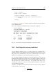
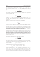
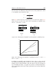
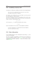
Figure 10.1 shows how these scalability laws are connected. Figure 10.2
shows how the speed of the code scales (according to Amdahl’s law)
when α = 0.02 and α = 0.002.
W
1
W
p
1–aa
W
1
W
p
/p
(1–a)/pa
1
W
1
pW
p
p(1–a')a'
W
1
W
p
(1–a')/pa'
1
Amdahl's
law
Gustafson's
law
Figure 10.1: Illustration of Amdahl’s and Gustafson’s scalability laws.
0 20 40 60 80 100 120 140
0
20
40
60
80
100
120
140
Figure 10.2: Illustration of Amdahl’s scalability law for α = 0.02 (−−)
and α = 0.002 (−·−).
In addition to Amdahl’s and Gustafson’s laws, there is also a model
for memory-bounded speedup. In this case the actual constraint is the
memory of the parallel machine, and you want to scale the program to
use all available memory. A typical case of this is 3D fluid mechanics,
where you usually want to solve large problems (dense grid) as efficiently
as possible.