Zoom out Search Issue

ManualsBrandsContents Manualsaudio & home theatreZoom in

151

152

153

154

155

156

157

158

159

160

IEEE SIGNAL PROCESSING MAGAZINE [158] MARCH 2015

PPtXG

()

() ()

## #g,

(17)

.QQuYG

()

() ()

## #g,

(18)

A number of data-analytic problems can be reformulated as either

regression or similarity analysis [analysis of variance (ANOVA),

autoregressive moving average modeling (ARMA), linear discri-

minant analysis (LDA), and canonical correlation analysis (CCA)],

so that both the matrix and tensor PLS solutions can be general-

ized across exploratory data analysis.

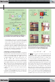
EXAMPLE 4

The predictive power of tensor-based PLS is illustrated on a real-

world example of the prediction of arm movement trajectory from

the electrocorticogram (ECoG). Figure 14(a) illustrates the experi-

mental setup, whereby the 3-D arm movement of a monkey was

captured by an optical motion capture system with reflective

markers affixed to the left shoulder, elbow, wrist, and hand; for full

details, see http://neurotycho.org. The predictors (32 ECoG chan-

nels) naturally build a fourth-order tensor

X (time#channel_no

# epoch_length # frequency) while the movement trajectories for

the four markers (response) can be represented as a third-order

tensor

Y (time# 3D_marker_position# marker_no). The goal of

the training stage is to identify the HOPLS parameters:

,,,PQGG

() ()

(see Figure 13). In the test stage, the move-

ment trajectories, ,Y

for the new ECoG data, ,X

are predicted

through multilinear projections: 1) the new scores, ,t

are found

from new data, ,X

and the existing model parameters:

,,,,PPPG

()

() () ()

rrr

123

and 2) the predicted trajectory is calculated as

.QQQtYG

()

() () ()

rrr

####.

In the simulations,

standard PLS was applied in the same way to the unfolded tensors.

Figure 14(c) shows that although the standard PLS was able

to predict the movement corresponding to each marker indi-

vidually, such a prediction is quite crude as the two-way PLS

does not adequately account for mutual information among the

four markers. The enhanced predictive performance of the BTD-

based HOPLS [the red line in Figure 14(c)] is therefore attrib-

uted to its ability to model interactions between complex latent

components of both predictors and responses.

LINKED MULTIWAY COMPONENT ANALYSIS

AND TENSOR DATA FUSION

Data fusion concerns the joint analysis of an ensemble of data

sets, such as multiple views of a particular phenomenon, where

some parts of the scene may be visible in only one or a few data

sets. Examples include the fusion of visual and thermal images

in low-visibility conditions and the analysis of human electro-

physiological signals in response to a certain stimulus but from

different subjects and trials; these are naturally analyzed

together by means of matrix/tensor factorizations. The coupled

nature of the analysis of such multiple data sets ensures that we

are able to account for the common factors across the data sets

and, at the same time, to guarantee that the individual compo-

nents are not shared (e.g., processes that are independent of exci-

tations or stimuli/tasks).

The linked multiway component analysis (LMWCA) [106],

shown in Figure 15, performs such a decomposition into shared

and individual factors and is formulated as a set of approxi-

mate joint TKD of a set of data tensors

,RX

()kIII

N12

## #g

(,,,)kK12f=

,BB BXG

() () (,) (,) ( ,)kk k k

## #g, (19)

where each factor matrix [, ]BBBR

(,)

()

(,)

has

1) components B R

()

(with )CR0

## that are common

(i.e., maximally correlated) to all tensors and 2) components

B R

(,)

()

IRC

nnn

# -

that are tensor specific. The objective is to esti-

mate the common components ,B

()

the individual components

(,)

and, via the core tensors ,G

()k

their mutual interactions. As

in MWCA (see the section “Tucker Decomposition”), constraints

may be imposed to match data properties [73], [76]. This enables a

more general and flexible framework than group ICA and independ-

ent vector analysis, which also performs linked analysis of multiple

data sets but assume that 1) there exist only common components

and 2) the corresponding latent variables are statistically independ-

ent [107], [108]. Both are quite stringent and limiting assumptions.

As an alternative to TKD, coupled tensor decompositions may be of

a polyadic or even block term type [89], [109].

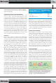
[FIG13] The principle of HOPLS for third-order tensors. The core

tensors G

and G

are block-diagonal. The BTD-type structure

allows for the modeling of general components that are highly

correlated in the first mode.

THE WORLD’S NEWSSTAND

THE WORLD’S NEWSSTAND

...

+ ··· +

(2)

× L

)

(2)

× L

)

(2)

× L

)

(2)

× RL

)

(1)T

(2)

× L

)

× I

)

(I )

× J

)

(J )

(I )

× I

)(L

× I

)

(RL

× I

)(R × RL

× RL

)

× R)

(2)

× RL

)

(1)T

(J )

× J

)(L

× J

)

(RL

× J

)(R × RL

× RL

)

× R)