Zoom out Search Issue

ManualsBrandsContents Manualsaudio & home theatreZoom in

151

152

153

154

155

156

157

158

159

160

IEEE SIGNAL PROCESSING MAGAZINE [156] MARCH 2015

possible to control the error and achieve any desired accuracy of

approximation. For example, tensor networks allow for the

representation of a wide class of discretized multivariate functions

even in cases where the number of function values is larger than

the number of atoms in the universe [23], [29], [30].

Examples of tensor networks are the hierarchical TKD and ten-

sor trains (TTs) (see Figure 9) [17], [18]. The TTs are also known as

matrix product states and have been used by physicists for more

than two decades (see [92] and [93] and references therein). The

PARATREE algorithm was developed in signal processing and fol-

lows a similar idea; it uses a polyadic representation of a data ten-

sor (in a possibly nonminimal number of terms), whose

computation then requires only the matrix SVD [94].

For very large-scale data that exhibit a well-defined structure,

an even more radical approach to achieve a parsimonious

representation may be through the concept of quantized or quan-

tic tensor networks (QTNs) [29], [30]. For example, a huge vector

x R

! with I 2

= elements can be quantized and tensorized

into a ()22 2## #g tensor X of order ,L as illustrated in Fig-

ure 2(a). If x is an exponential signal, ( ) ,xk az

= then X is a

symmetric rank-1 tensor that can be represented by two parame-

ters: the scaling factor

a and the generator z (cf. (2) in the sec-

tion “Tensorization—Blessing of Dimensionality”). Nonsymmetric

terms provide further opportunities, beyond the sum-of-exponen-

tial representation by symmetric low-rank tensors. Huge matrices

and tensors may be dealt with in the same manner. For instance,

Nth-order tensor ,RX

##g

with ,I q

= can be quan-

tized in all modes simultaneously to yield a ()qq q## #g

quantized tensor of higher order. In QTN, q is small, typically

,,,q 234= e.g., the binary encoding q 2=

reshapes an Nth

-order tensor with ()22 2

LL L

N12

###g elements into a tensor

of order ()LL L

N12

g++ + with the same number of elements.

The TT decomposition applied to quantized tensors is referred to

as the quantized TT (QTT); variants for other tensor representa-

tions have also been derived [29], [30]. In scientific computing,

such formats provide the so-called supercompression—a logarith-

mic reduction of storage requirements:

.() ( ())logI N IOO

COMPUTATION OF THE

DECOMPOSITION/REPRESENTATION

Now that we have addressed the possibilities for efficient tensor rep-

resentation, the question that needs to be answered is how these

representations can be computed from the data in an efficient man-

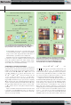
ner. The first approach is to process the data in smaller blocks

rather than in a batch manner [95]. In such a divide-and-conquer

approach, different blocks may be processed in parallel, and their

decompositions may be carefully recombined (see Figure 10) [95],

[96]. In fact, we may even compute the decomposition through

recursive updating as new data arrive [97]. Such recursive tech-

niques may be used for efficient computation and for tracking

decompositions in the case of nonstationary data.

The second approach would be to employ CS ideas (see the sec-

tion “Higher-Order Compressed Sensing (HO-CS)”) to fit an alge-

braic model with a limited number of parameters to possibly large

data. In addition to enabling data completion (interpolation of

missing data), this also provides a significant reduction of the cost

of data acquisition, manipulation, and storage, breaking the curse

of dimensionality being an extreme case.

While algorithms for this purpose are available both for low-

rank and low multilinear rank representation [59], [87], an even

more drastic approach would be to directly adopt sampled fibers

as the bases in a tensor representation. In the TKD setting, we

would choose the columns of the factor matrices

()n

mode-n fibers of the tensor, which requires us to address the fol-

lowing two problems: 1) how to find fibers that allow us to accurately

represent the tensor and 2) how to compute the corresponding core

tensor at a low cost (i.e., with minimal access to the data). The mat-

rix counterpart of this problem (i.e., representation of a large

matrix on the basis of a few columns and rows) is referred to as

the pseudoskeleton approximation [98], where the optimal

representation corresponds to the columns and rows that inter-

sect in the submatrix of maximal volume (maximal absolute

value of the determinant). Finding the optimal submatrix is

computationally hard, but quasioptimal submatrices may be

found by heuristic so-called cross-approximation methods that

(k)

(1)

(k)

(K)

(1)

(k )

(K )

......

(1)

(k)

(K )

(1)

(k)

(K )

(K )T

(k )T

(1)T

∼

[FIG10] Efficient computation of CPD and TKD, whereby tensor decompositions are computed in parallel for sampled blocks. These are

then merged to obtain the global components A, B, and C, and a core tensor .G

THE WORLD’S NEWSSTAND

THE WORLD’S NEWSSTAND