Zoom out Search Issue

ManualsBrandsContents Manualsaudio & home theatreZoom in

151

152

153

154

155

156

157

158

159

160

IEEE SIGNAL PROCESSING MAGAZINE [155] MARCH 2015

[85]. The Kronecker-CS model has been applied in magnetic res-

onance imaging, hyperspectral imaging, and in the inpainting of

multiway data [86], [84].

APPROACHES WITHOUT FIXED DICTIONARIES

In Kronecker-CS, the modewise dictionaries

B R

()nII

can be

chosen so as best to represent the physical properties or prior

knowledge about the data. They can also be learned from a large

ensemble of data tensors, for instance, in an ALS-type fashion

[86]. Instead of the total number of sparse entries in the core ten-

sor, the size of the core (i.e., the multilinear rank) may be used as

a measure for sparsity so as to obtain a low-complexity represen-

tation from compressively sampled data [87], [88]. Alternatively, a

CPD representation can be used instead of a Tucker representa-

tion. Indeed, early work in chemometrics involved excitation–

emission data for which part of the entries was unreliable because

of scattering; the CPD of the data tensor is then computed by

treating such entries as missing [7]. While CS variants of several

CPD algorithms exist [59], [89], the oracle properties of tensor-

based models are still not as well understood as for their standard

models; a notable exception is CPD with sparse factors [90].

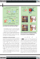
EXAMPLE 3

Figure 8 shows an original 3-D (1,024

# 1,024 # 32) hyperspectral

image ,X which contains scene reflectance measured at 32 differ-

ent frequency channels, acquired by a low-noise Peltier-cooled dig-

ital camera in the wavelength range of 400–720 nm [91]. Within

the Kronecker-CS setting, the tensor of compressive measure-

ments

Y was obtained by multiplying the frontal slices

by random Gaussian sensing matrices R

() M11024

and

() M21024

(, , )MM 1024

1 in the first and second mode,

respectively, while R

()33232

was the identity matrix [see

Figure 8(a)]. We used Daubechies wavelet factor matrices

BBR

() ()1 2 1024 1024

and ,B R

()33232

and employed the

N-way block tensor N-BOMP to recover the small sparse core tensor

and, subsequently, reconstruct the original 3-D image, as shown

in Figure 8(b). For the sampling ratio SP

= 33% ( )MM585

this gave the peak SNR (PSNR) of 35.51 dB, while taking 71 min

for

N 841

iter

= iterations needed to detect the subtensor which

contains the most significant entries. For the same quality of

reconstruction (PSNR= 35.51 dB), the more conventional

Kronecker-OMP algorithm found 0.1% of the wavelet coefficients

as significant, thus requiring

.(,NK0 001 1 024

iter

##==

,),1024 32 33 555# = iterations and days of computation time.

LARGE-SCALE DATA AND THE CURSE OF DIMENSIONALITY

The sheer size of tensor data easily exceeds the memory or satu-

rates the processing capability of standard computers; it is, there-

fore, natural to ask ourselves how tensor decompositions can be

computed if the tensor dimensions in all or some modes are large

or, worse still, if the tensor order is high. The term curse of

dimensionality, in a general sense, was introduced by Bellman to

refer to various computational bottlenecks when dealing with

high-dimensional settings. In the context of tensors, the curse of

dimensionality refers to the fact that the number of elements of an

Nth-order ( )II I## #g tensor, ,I

scales exponentially with

the tensor order .N For example, the number of values of a discre-

tized function in Figure 2(b) quickly becomes unmanageable in

terms of both computations and storing as

N increases. In addi-

tion to their standard use (signal separation, enhancement, etc.),

tensor decompositions may be elegantly employed in this context

as efficient representation tools. The first question is, which type

of tensor decomposition is appropriate?

EFFICIENT DATA HANDLING

If all computations are performed on a CP representation and not

on the raw data tensor itself, then, instead of the original

raw

data entries, the number of parameters in a CP representation

reduces to

,NIR which scales linearly in N (see Table 4). This

effectively bypasses the curse of dimensionality, while giving us the

freedom to choose the rank,

,R as a function of the desired accuracy

[16]; on the other hand, the CP approximation may involve numer-

ical problems (see the section “Canonical Polyadic Decomposition”).

Compression is also inherent to TKD as it reduces the size of a

given data tensor from the original

to ( ),NIR R

+ thus exhib-

iting an approximate compression ratio of .(/ )IR

We can then

benefit from the well understood and reliable approximation by

means of matrix SVD; however, this is only useful for low

TENSOR NETWORKS

A numerically reliable way to tackle curse of dimensionality is

through a concept from scientific computing and quantum infor-

mation theory, termed tensor networks, which represents a tensor

of a possibly very high order as a set of sparsely interconnected

matrices and core tensors of low order (typically, order 3). These

low-dimensional cores are interconnected via tensor contractions

to provide a highly compressed representation of a data tensor. In

addition, existing algorithms for the approximation of a given ten-

sor by a tensor network have good numerical properties, making it

[TABLE 4] STORAGE COST OF TENSOR MODELS FOR AN

thN -ORDER TENSOR RX

II I

## #g

FOR WHICH THE STORAGE

REQUIREMENT FOR RAW DATA IS ( ).IO

1) CANONICAL POLYADIC DECOMPOSITION

()NIRO

2) TUCKER

()NIR RO

3) TENSOR TRAIN

()NIRO

4) QUANTIZED TENSOR TRAIN

(())logNR IO

THE WORLD’S NEWSSTAND

THE WORLD’S NEWSSTAND

× R

)

× l

× R

)

× l

× R

)

× l

× R

)

× l

)

(1)

(2)

(3)

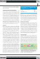
[FIG9] The TT decomposition of a fifth-order tensor ,RX

II I

12 5

## #g

consisting of two matrix carriages and three third-order tensor

carriages. The five carriages are connected through tensor

contractions, which can be expressed in a scalar form as x

,,,,iiiii

12345

agggb.

()

rir rir rir

123

122 233 345

===

///