Zoom out Search Issue

ManualsBrandsContents Manualsaudio & home theatreZoom in

151

152

153

154

155

156

157

158

159

160

IEEE SIGNAL PROCESSING MAGAZINE [149] MARCH 2015

tensor. The tensor rank is defined as the smallest value of R for

which (3) holds exactly; the minimum rank PD is called canoni-

cal PD (CPD) and is desired in signal separation. The term CPD

may also be considered as an abbreviation of CANDECOMP/

PARAFAC decomposition, see the “Historical Notes” section. The

matrix/vector form of CPD can be obtained via the Khatri–Rao

products (see Table 2) as

,XBDB B B B

()

() () () () ()

nN n n

11 1

99 9 99gg=

() [ ],BB Bdvec X

() ( ) ()NN11

999g=

(5)

where .,,,[]d

fmm m=

RANK

As mentioned earlier, the rank-related properties are very

different for matrices and tensors. For instance, the number of

complex-valued rank-1 terms needed to represent a higher-order

tensor can be strictly smaller than the number of real-valued

rank-1 terms [22], while the determination of tensor rank is in gen-

eral NP-hard [41]. Fortunately, in signal processing applications,

rank estimation most often corresponds to determining the num-

ber of tensor components that can be retrieved with sufficient

accuracy, and often there are only a few data components present.

A pragmatic first assessment of the number of components may be

through inspection of the multilinear singular value spectrum (see

the “Tucker Decomposition” section), which indicates the size of

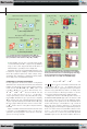
the core tensor in the right-hand side of Figure 3(b). The existing

techniques for rank estimation include the core consistency diag-

nostic (CORCONDIA) algorithm, which checks whether the core

tensor is (approximately) diagonalizable [7], while a number of

techniques operate by balancing the approximation error versus

the number of degrees of freedom for a varying number of rank-1

terms [42]–[44].

UNIQUENESS

Uniqueness conditions give theoretical bounds for exact tensor

decompositions. A classical uniqueness condition is due to Kruskal

[33], which states that for third-order tensors, the CPD is unique up

to unavoidable scaling and permutation ambiguities, provided that

,kkk R22

BBB

() () ()123

$++ + where the Kruskal rank k

of a matrix

B is the maximum value ensuring that any subset of k

columns is

linearly independent. In sparse modeling, the term ()k 1

+ is also

known as the spark [32]. A generalization to Nth-order tensors is

due to Sidiropoulos and Bro [45] and is given by

.k R N21

()n

$ +-

(6)

More relaxed uniqueness conditions can be obtained when one

factor matrix has full-column rank [46]–[48]; for a thorough

study of the third-order case, we refer to [34]. This all shows that,

compared to matrix decompositions, CPD is unique under more

natural and relaxed conditions, which only require the compo-

nents to be sufficiently different and their number not unreason-

ably large. These conditions do not have a matrix counterpart and

are at the heart of tensor-based signal separation.

COMPUTATION

Certain conditions, including Kruskal’s, enable explicit computa-

tion of the factor matrices in (3) using linear algebra [essentially,

by solving sets of linear equations and computing (generalized)

EVD] [6], [47], [49], [50]. The presence of noise in data means

that CPD is rarely exact, and we need to fit a CPD model to the

data by minimizing a suitable cost function. This is typically

achieved by minimizing the Frobenius norm of the difference

between the given data tensor and its CP approximation, or, alter-

natively, by least absolute error fitting when the noise is Lapla-

cian [51]. The theoretical Cramér–Rao lower bound and

[FIG3] The analogy between (a) dyadic decompositions and (b) PDs; the Tucker format has a diagonal core. The uniqueness of these

decompositions is a prerequisite for BSS and latent variable analysis.

THE WORLD’S NEWSSTAND

THE WORLD’S NEWSSTAND

+ ··· +

(I × J )

(R × J )(R × R )(I × R )

∼

(a)

+ ··· +

(I × J × k )

(K × R )

(R × J )(R × R × R )(I × R )

(b)