Zoom out Search Issue

ManualsBrandsContents Manualsaudio & home theatreZoom in

121

122

123

124

125

126

127

128

129

130

IEEE SIGNAL PROCESSING MAGAZINE [127] MARCH 2015

of Figure 1. Intuitively, the signal is entirely composed of only two

notes, and an effective decomposition technique would discover

these notes when they were played. PCA and ICA were employed

to decompose the spectrogram into two bases and their activa-

tions. In both cases, a nearly perfect decomposition is achieved in

the sense that the bases, when excited by their corresponding

activations, combine to construct the original spectrogram nearly

perfectly, reflecting the fact that the signal does indeed comprise

only two basic elements (i.e., the two notes). However, an inspec-

tion of the actual bases discovered and their activations reveals a

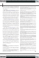
problem. PCA [see Figure 2(a)] discovers two bases that, although

orthogonal to one another, are actually combinations of the two

notes, and their corresponding activations provide no indication

of the actual composition of the sound. In this particular example,

ICA [see Figure 2(a)] discovers two bases whose activations track

the actual activation of the notes in the signal. However, the dis-

covered bases themselves have both negative and positive compo-

nents, effectively characterizing the atomic units that compose

the sound as having negative spectral magnitudes, which has no

physical interpretation. More generally, even the degree of con-

formance to the underlying structure found in this particular

example is usually not achieved. The intuitive dissonance is obvi-

ous—intuitively, the building blocks of this sound were the notes

and both methods have failed to discover these effectively.

Although we do not go into this further, the dissonance is more

than intuitive; several of the solutions we develop later in

the article through compositional models are simply not

possible through normal matrix decomposition techniques

such as PCA and ICA, which permit both constructive and

destructive composition.

In contrast, Figure 3 shows the results obtained by decom-

posing the spectrogram of Figure 1 with NMF. The nonnegative

factorization is observed to successfully uncover both the notes

themselves (as defined by their spectra) and their activations. In

practice, the discovered atoms will not always have as clearly

associative semantics as in this example; for instance, in

Figure 3, we have assumed that the correct number of atoms, two,

is known a priori, and this is generally not the case. Neverthe-

less, the atoms that are discovered tend to be consistent spectral

structures that compose the signal.

REPRESENTING AUDIO SIGNALS

As noted earlier, the constructive compositionality of sound is

evidenced in the distribution of energy in time–frequency char-

acterizations of the signal. This observation has a theoretical

basis: the power in any frequency band of the sum of uncorre-

lated signals is the sum of the powers of the individual signals

within that band. We will therefore employ time–frequency

characterizations to represent audio signals.

The time–frequency characterizations of the signal are gener-

ally obtained through filter bank analysis. Thus, a signal

[],yn

nN1g= is transformed into a matrix of values [ , ],Ytf t=

,,Tf F11gg= where T is the number of time frames, F is the

number of filters in the filter bank, and /NT

x =

is the period

with which the output of the filter bank is sampled. It is also

(a)

−0.8 0

PCA

Atom 1

Frequency (kHz)

−1 0 0.5

PCA

Atom 2

−0.2 0

ICA

Atom 1

0 0.2

ICA

Atom 2

−4

−2

PCA Activation 1

(b)

1 2 3

−3

−2

−1

PCA Activation 2

Time (s)

−3

−2

−1

ICA Activation 1

1 2 3

ICA Activation 2

Time (s)

[FIG2] The PCA and ICA analyses of the data in Figure 1:

(a) the learned PCA and ICA atoms and (b) their corresponding

activations. Compared to the learned parameters in Figure 3,

we can see that these analyses are not resulting in an intuitive

decomposition.

Atom 1

Frequency (kHz)

Atom 2

0.5 1 1.5 2 2.5 3 3.5

0.5

Activation 2

Time (s)

0.5 1 1.5 2 2.5 3 3.5

Time (s)

(c)

0.5

Activation 1

(b)(a)

Approximation to Input

[FIG3] The NMF decomposition of the spectrogram of Figure 1:

(a) the discovered atoms and (c) their corresponding activations

and (b) is the approximation to the input.

THE WORLD’S NEWSSTAND

THE WORLD’S NEWSSTAND