Zoom out Search Issue

ManualsBrandsContents Manualsaudio & home theatreZoom in

121

122

123

124

125

126

127

128

129

130

IEEE SIGNAL PROCESSING MAGAZINE [126] MARCH 2015

also the flexibility to use them in

ways that are nonstandard in audio

processing. In this article, we show

how they can be powerful tools for

processing audio data, providing

highly interpretable audio represen-

tations and enabling diverse applica-

tions such as signal analysis and

recognition [4], [7], [8], manipula-

tion and enhancement [9], [10], and coding [11], [12].

The basic premise underlying the application of compositional

models to audio processing is that sound, too, can be viewed as

being compositional in nature. The premise has intuitive appeal:

sound, as we experience it, does indeed have compositional char-

acter. The sounds we hear are usually a medley of component

sounds that are all concurrently present. Although a sound may

mask others by its greater prominence, the sounds themselves do

not generally cancel one another, except in a few cases when it is

done intentionally, e.g., in adaptive noise cancellers. Even sounds

produced by a single source are often compositions of component

sounds from the source, e.g., the sound produced by a machine

combines sounds from all of its parts, and music sounds are com-

positions of notes produced by various instruments.

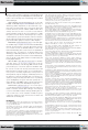
The compositionality of sound is also evident in time–

frequency characterizations of the signal, as illustrated by

Figure 1. The figure shows a spectrogram—a visual representa-

tion of the magnitude of time–frequency components as a func-

tion of time and frequency—of a signal, which comprises two

notes played individually at first and then played together. The

spectral patterns characteristic of the individual notes are dis-

tinctly observable even when they are played together.

The compositional framework for

sound analysis builds upon these

impressions: it characterizes the

sounds from any source as a con-

structive composition of atomic

sounds that are characteristic of the

source and postulates that the

decomposition of the signal into its

atomic parts may be achieved

through the application of an appropriately constrained compos-

itional model to an appropriate time–frequency representation of

the signal. This, in turn, can be used to perform several of the

tasks mentioned earlier.

The models themselves may take multiple forms. The

nonnegative matrix factorization (NMF) models [3], [13] treat

nonnegative time–frequency representations of the signal as

matrices, which are decomposed into products of nonnegative

component matrices. One of the matrices represents spectral

patterns of the atomic parts, and the other represents their acti-

vation to the signal over time.

The probabilistic latent component analysis (PLCA) models

treat the nonnegative time–frequency representations as histo-

grams drawn from a mixture of multivariate multinomial ran-

dom variables representing the atomic parts [14]. The two

approaches can be shown to be equivalent as well as arithmetic-

ally identical under some circumstances [15].

The purpose of this article is to serve as an introduction to the

application of compositional models to the analysis of sound. We

first demonstrate the limitations of related algorithms that allow

for the cancellation of parts and how compositional models can

circumvent them, through an example. We then continue with a

brief exposition on the type of time–frequency representations

where compositional models may naturally be applied.

We subsequently explain the models themselves. Two of the

most common formulations of compositional models are based

on matrix factorization and PLCA. For brevity, we primarily pre-

sent the matrix factorization perspective, although we also

introduce the PLCA model briefly for completeness.

Within these frameworks, we address various issues, including

how a given sound may be decomposed into the contributions of

its atomic parts, how the parts themselves may be found, restric-

tions of the model vis-à-vis the number and nature of these parts

and of the decomposition itself, and finally how the solutions to

these problems make various applications possible.

WHY CONSTRUCTIVE COMPOSITION?

Before proceeding further, it may be useful to address a question

that may already have struck you. Since the models themselves

are effectively matrix decompositions, what makes the compos-

itional model with its constraints on purely constructive compos-

ition different from other forms of matrix decompositions such as

principal component analysis (PCA), independent component

analysis (ICA), or other similar methods?

The answer is given as illustrated in Figure 2, which shows the

outcome of PCA- and ICA-based decomposition of the spectrogram

Time (s)

Frequency (kHz)

Magnitude Spectrogram

1 2 3

0.5

1.5

2.5

3.5

4.5

0.1

0.2

0.3

0.4

0.5

0.6

0.7

0.8

0.9

[FIG1] A magnitude spectrogram of a simple piano recording.

Two notes are played in succession and then again in unison.

We can visually identify these notes using their unique

harmonic structure.

THE BASIC PREMISE

UNDERLYING THE APPLICATION

OF COMPOSITIONAL MODELS

TO AUDIO PROCESSING IS THAT

SOUND CAN BE VIEWED AS BEING

COMPOSITIONAL IN NATURE.

THE WORLD’S NEWSSTAND

THE WORLD’S NEWSSTAND