User guide

Charnwood Dynamics Ltd. Coda cx1 User Guide – Advanced Topics III - 2
CX1 USER GUIDE - COMPLETE.doc 26/04/04 99/162
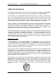
Whereas the first option is a secure definition (provided that the two chosen points never
coincide), the security of the second (planar definition) depends on the three chosen points
remaining ‘well separated’ throughout the data sequence; and in this case, well separated
means non co-linear as well as non co-incident (three points in a straight line do not
represent a plane). Due care must be taken when defining a vector by the latter option.
The second of our vectors may be defined in any of the ways described for the first vector
(though, obviously, it ought to be a different vector) or, alternatively, it may be defined as a
representation of any of the laboratory co-ordinate frame axes or the direction of subject
travel (presumed to be along the X axis). The latter alternative obviates the need to specify
any reference points or markers since co-ordinate axis vectors are known implicitly.
Vectors on Stick Figures
Whereas a vector defined between two markers is easily visualized using a Stick Figure
connection, a plane-normal vector cannot be similarly visualized unless an appropriately
located Virtual Marker is created with an ‘out-of-plane’ offset. (See Section: Virtual Markers.)
The Virtual Marker is made available to the markers list in the Stick Figure Joins Setup
dialogue box so that a connecting line can be shown on the figure.
Having defined two vectors one should proceed to choose the angle-type option; this will
depend on the purpose one has in mind.
3D Vector Angles
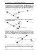
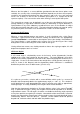
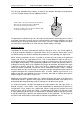
A ‘3D’ vector angle is calculated by means of the inverse cosine (trigonometric) function
applied to the scalar (“dot”) product of the two vectors. The angle obtained is that which
would be measured by a protractor if the two vectors were brought together to intersect in a
single point. Of course, the intersection of two straight lines actually presents two angles (α
and β as shown in the diagram) and the trigonometry obtains whichever is sandwiched
between the positive senses of both vectors (β in this case).
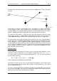
It is quite easy to make a mistake with a vector definition which results in a reversal of
direction and consequently obtains the supplementary angle (α = 180
o
- β). This situation is
easily identified on a graph plot provided the angle in question varies from an approximate,
fixed right-angle. It is easily rectified by reversing one of the vector definitions.
Note that the trigonometric derivation of 3D angles delivers values in the range 0
o
to 180
o
only. In particular the angle is always non-negative and should be regarded as an absolute
angle between vectors. The 3D angle is, therefore, unsuitable for observing angles expected
to vary from positive to negative (for example - foot attitude relative to the floor): instead of
progressing from positive, through zero, into the negative range, the graph plot would show a
characteristic ‘bounce’ from the abscissa. (Likewise, circular motions would not proceed
beyond 180
o
, but bounce back and forth within the plotable range.)
β
β
ββ
β
α
α