User guide

Charnwood Dynamics Ltd. Coda cx1 User Guide – Advanced Topics III - 3
CX1 USER GUIDE - COMPLETE.doc 26/04/04 103/162
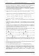
One way would be to look at the projections of distal axes onto the axial planes of the
proximal co-ordinate frame. The angles between proximal axes and corresponding
projections of distal axes are called Projection Angles (there are 8 possible sets!)
5
and
although these are definitely NOT the same as Euler Angles there is a useful
correspondence between the two types (as we shall see later) and many clinicians will
already be familiar with the notion of angles ‘projected’ onto the sagittal plane. The
calculation of these projection angles is more intuitively obvious (they can be measured
with a protractor on projected views); so why not adopt this scheme?
Unfortunately, projection angles do not describe rotations of the segment about clinically
relevant axes and it is here that Euler schemes take the lead.
Euler Angles are readily calculated (requiring no joint centre model), and correspond to
quite relevant axes which are generally orthogonal and therefore kinetically useful.
In recent years there has been much debate on the relative merits of various ‘Euler’
schemes, some of which employ anatomically skewed axes at the expense of
orthogonality and generality. (One such scheme, the ‘Joint Co-ordinate System’ of Grood
and Suntay (1983)
6
scores highly for some joint geometries, such as the knee, but the
non-orthogonal nature of the axes is a limiting factor.)
The (orthogonal) scheme described here is widely accepted as providing consistently
appropriate descriptions of most segment-joint geometries along with suitable derivatives
for kinetic purposes.
Eulerian System
Consider a distal limb segment initially in the ‘neutral’ position, such that its EVB axes
coincide exactly with those of the proximal segment. Clearly the Euler Angles are all zero
for this situation but if, at some other instant, the distal segment is re-positioned elsewhere
the new set of Euler Angles ought to quantify the necessary rotations (about the proximal
axes) by which it arrives there.
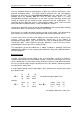
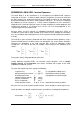
A single rotation through a given angle about a given (proximal) axis may be represented
by a rotation matrix:
| 1 0 0 |
R
x
= | 0 cosθ −sinθ | for rotation through θ about X axis.
| 0 sinθ cosθ |
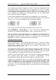
Similarly,
| cosφ 0 sinφ | | cosψ -sinψ 0 |
R
y
= | 0 1 0 | and R
z
= | sinψ cosψ 0 |
| - sinφ 0 cosφ | | 0 0 1 |
for rotations about the Y and Z axes.