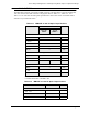
Technical data

TraverseEdge 2020 Applications and Engineering Guide, Chapter 7: Optical Link Design
Page 7-14 Turin Networks Release 5.0.x
For the reasons listed above, the variance between calculated and actual attenuation on a given
span can be quite high. Therefore, Turin Networks recommends measuring the actual attenua-
tion for each link if and where possible.
Chromatic Dispersion (D
T
)
Chromatic dispersion is a result of the variance in group-velocity with frequency. Each output
pulse from a laser source, though generally considered to be of a single wavelength or frequency,
is actually composed of a spectrum of wavelengths. As the pulse travels along the fiber the higher
frequency components (shorter wavelengths) travel faster than the lower frequency (longer wave-
length components), the result being: pulse broadening. With sufficient pulse broadening, each
pulse will begin to interfere with neighboring (ahead or behind) pulse, distorting the transmission
signal.
As the speed of transmission increases the individual pulses are necessarily close together and,
therefore, less tolerant of dispersion. Although combating dispersions is possible by narrowing the
spectral width of each pulse, the returns of this approach rapidly diminish with the ratio of spectral
and inter-digital time. In fact, spectral width being constant, chromatic dispersion increases with
the square of the bit-rate. For example, moving from 2.5Gbps to 10Gbps, a 4X increase in bit-rate,
results in a 16X increase in chromatic dispersion. Since dispersion is never the limiting factor in
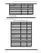
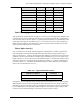
optical budgeting at OC-3 and OC-12 rates, only Table 7-4 through Table 7-13 for OC-48 and
OC-192 Optical Parameters includes dispersion values.
System Margin (M)
In an optical link design, planners generally leave room for a Margin of Error, generally referred to
as System Margin or simply Margin. This margin is justified primarily as a safeguard to ensure
links will continue to operate as changes to the fiber plant in the future. Such changes could
include adding a new LDF in-line and/or new splices (e.g., when making repairs to damaged
fiber). While some network operators use a system margin as high as 5dB, the more typical value
of 3dB is used in all example link budgets in this document.
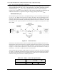
7.3 Calculating Single-Span Fiber Link Budgets
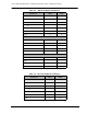
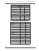
With a basic understanding of the parameters defined above and the information provided in
Table 7-1 through Table 7-13 , optical link budgets may be computed for almost any ‘real world’
scenario. The basic process of link budgeting begins with the transceiver power budget, P
T
of a
given transmitter/receiver pair, that is, the difference between P
tmin
and P
rmin
. The known sources
of loss (i.e., connector losses and margin) are subtracted from the transceiver power budget, the
difference being the fiber link power budget, P
f
. The fiber link power budget is essentially the
budget allowable to cable loss (including splices and additional connectors).
P
T
= P
tmin
- P
rmin
P
f
= P
T
- L
c
- M
Determining the fiber link power budget is an important first step in optical span design. Further
steps require information relating to the actual fiber plant targeted for use. Two key parameters
(measured or calculated based on fiber cable manufacturers’ data) relating to the fiber plant are