
User's Manual
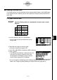
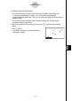
Table Of Contents
- Quick-Start
- Precautions when Using this Product
- Contents
- Getting Acquainted— Read This First!
- Chapter 1 Basic Operation
- Chapter 2 Manual Calculations
- Chapter 3 List Function
- Chapter 4 Equation Calculations
- Chapter 5 Graphing
- 5-1 Sample Graphs
- 5-2 Controlling What Appears on a Graph Screen
- 5-3 Drawing a Graph
- 5-4 Storing a Graph in Picture Memory
- 5-5 Drawing Two Graphs on the Same Screen
- 5-6 Manual Graphing
- 5-7 Using Tables
- 5-8 Dynamic Graphing
- 5-9 Graphing a Recursion Formula
- 5-10 Changing the Appearance of a Graph
- 5-11 Function Analysis
- Chapter 6 Statistical Graphs and Calculations
- Chapter 7 Financial Calculation (TVM)
- Chapter 8 Programming
- Chapter 9 Spreadsheet
- Chapter 10 eActivity
- Chapter 11 System Settings Menu
- Chapter 12 Data Communications
- Appendix
20070201
9-6-3
Statistical Graphs
k Graphing Statistical Data
The following shows an actual example of how to graph statistical data in the S
•
SHT mode.
It also explains various methods you can use to specify the range of cells that contains the
graph data.
u To graph statistical data
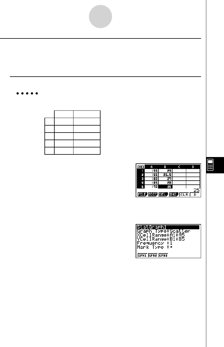
Example: Input the following data into a spreadsheet, and then draw a scatter
diagram.
Height Shoe Size
A 155 23
B 165 25.5
C 180 27
D 185 28
E 170 25
1. Input the statistical data into a spreadsheet.
• Here, we will input the above data into the cell
range A1:B5.
2. Select the cell ranges you want to graph.
• Here we will select the range A1:B5.
3. Press 6 (g )1 (GRPH) to display the GRPH submenu.
4. Press 6 (SET).
• This displays the StatGraph1 settings screen. The
fi rst column of cells you selected in step 2 will
be displayed for XCellRange, while the second
column will be displayed for YCellRange.
• You can change the XCellRange and YCellRange settings manually, if you want. For
details, see “Confi guring Range Settings for Graph Data Cells” (page 9-6-5).