
User's Manual
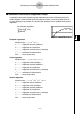
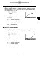
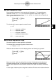
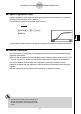
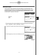
Table Of Contents
- Quick-Start
- Precautions when Using this Product
- Contents
- Getting Acquainted— Read This First!
- Chapter 1 Basic Operation
- Chapter 2 Manual Calculations
- Chapter 3 List Function
- Chapter 4 Equation Calculations
- Chapter 5 Graphing
- 5-1 Sample Graphs
- 5-2 Controlling What Appears on a Graph Screen
- 5-3 Drawing a Graph
- 5-4 Storing a Graph in Picture Memory
- 5-5 Drawing Two Graphs on the Same Screen
- 5-6 Manual Graphing
- 5-7 Using Tables
- 5-8 Dynamic Graphing
- 5-9 Graphing a Recursion Formula
- 5-10 Changing the Appearance of a Graph
- 5-11 Function Analysis
- Chapter 6 Statistical Graphs and Calculations
- Chapter 7 Financial Calculation (TVM)
- Chapter 8 Programming
- Chapter 9 Spreadsheet
- Chapter 10 eActivity
- Chapter 11 System Settings Menu
- Chapter 12 Data Communications
- Appendix
20070201
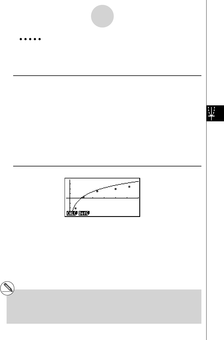
Example Input the two sets of data shown below. Next, plot the data on a scatter
diagram and overlay a function graph
y = 2ln x .
0.5, 1.2, 2.4, 4.0, 5.2
–2.1, 0.3, 1.5, 2.0, 2.4
Procedure
1 m STAT
2 a.f w b.c w
c.e w e w f.c w
e
- c.b w a.d w
b.f w c w c.e w
1 (GRPH)1 (GPH1)
3 2 (DefG)
c Ivw (Register Y1 = 2In
x )
4 6 (DRAW)
Result Screen
6-3-14
Calculating and Graphing Paired-Variable Statistical Data
# You can also perform trace, etc. for drawn
function graphs.
# Graphs of types other than rectangular
coordinate graphs cannot be drawn.
# Pressing J while inputting a function returns
the expression to what it was prior to input.
Pressing !J (QUIT) clears the input
expression and returns to the statistical data list.