
User Manual
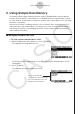
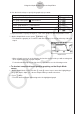
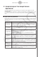
Table Of Contents
- Contenu
- Familiarisation — A lire en premier!
- Chapitre 1 Opérations de base
- Chapitre 2 Calculs manuels
- 1. Calculs de base
- 2. Fonctions spéciales
- 3. Spécification de l’unité d’angle et du format d’affichage
- 4. Calculs de fonctions
- 5. Calculs numériques
- 6. Calculs avec nombres complexes
- 7. Calculs binaire, octal, décimal et hexadécimal avec entiers
- 8. Calculs matriciels
- 9. Calculs vectoriels
- 10. Calculs de conversion métrique
- Chapitre 3 Listes
- Chapitre 4 Calcul d’équations
- Chapitre 5 Représentation graphique de fonctions
- 1. Exemples de graphes
- 2. Contrôle des paramètres apparaissant sur un écran graphique
- 3. Tracé d’un graphe
- 4. Stockage d’un graphe dans la mémoire d’images
- 5. Tracé de deux graphes sur le même écran
- 6. Représentation graphique manuelle
- 7. Utilisation de tables
- 8. Représentation graphique dynamique
- 9. Représentation graphique d’une formule de récurrence
- 10. Tracé du graphe d’une section conique
- 11. Changement de l’aspect d’un graphe
- 12. Analyse de fonctions
- Chapitre 6 Graphes et calculs statistiques
- 1. Avant d’effectuer des calculs statistiques
- 2. Calcul et représentation graphique de données statistiques à variable unique
- 3. Calcul et représentation graphique de données statistiques à variable double
- 4. Exécution de calculs statistiques
- 5. Tests
- 6. Intervalle de confiance
- 7. Lois de probabilité
- 8. Termes des tests d’entrée et sortie, intervalle de confiance et loi de probabilité
- 9. Formule statistique
- Chapitre 7 Calculs financiers
- 1. Avant d’effectuer des calculs financiers
- 2. Intérêt simple
- 3. Intérêt composé
- 4. Cash-flow (Évaluation d’investissement)
- 5. Amortissement
- 6. Conversion de taux d’intérêt
- 7. Coût, prix de vente, marge
- 8. Calculs de jours/date
- 9. Dépréciation
- 10. Calculs d’obligations
- 11. Calculs financiers en utilisant des fonctions
- Chapitre 8 Programmation
- 1. Étapes élémentaires de la programmation
- 2. Touches de fonction du mode PROGR (ou PRGM)
- 3. Édition du contenu d’un programme
- 4. Gestion de fichiers
- 5. Guide des commandes
- 6. Utilisation des fonctions de la calculatrice dans un programme
- 7. Liste des commandes du mode PROGR (ou PRGM)
- 8. Tableau de conversion des commandes spéciales de la calculatrice scientifique CASIO <=> Texte
- 9. Bibliothèque de programmes
- Chapitre 9 Feuille de Calcul
- Chapitre 10 L’eActivity
- Chapitre 11 Gestionnaire de la mémoire
- Chapitre 12 Menu de réglages du système
- Chapitre 13 Communication de données
- Chapitre 14 PYTHON
- 1. Aperçu du mode PYTHON
- 2. Menu de fonctions de PYTHON
- 3. Saisie de texte et de commandes
- 4. Utilisation du SHELL
- 5. Utilisation des fonctions de tracé (module casioplot)
- 6. Modification d’un fichier py
- 7. Gestion de dossiers (recherche et suppression de fichiers)
- 8. Compatibilité de fichier
- 9. Exemples de scripts
- Chapitre 15 Probabilités
- Appendice
- Mode Examen
- E-CON3 Application (English) (GRAPH35+ E II)
- 1 E-CON3 Overview
- 2 Using the Setup Wizard
- 3 Using Advanced Setup
- 4 Using a Custom Probe
- 5 Using the MULTIMETER Mode
- 6 Using Setup Memory
- 7 Using Program Converter
- 8 Starting a Sampling Operation
- 9 Using Sample Data Memory
- 10 Using the Graph Analysis Tools to Graph Data
- 11 Graph Analysis Tool Graph Screen Operations
- 12 Calling E-CON3 Functions from an eActivity

11 Graph Analysis Tool Graph Screen
Operations
This section explains the various operations you can perform on the graph screen after
drawing a graph.
You can perform these operations on a graph screen produced by a sampling operation, or by
the operation described under “Selecting an Analysis Mode and Drawing a Graph” on page
10-2.
k Graph Screen Key Operations
On the graph screen, you can use the keys described in the table below to analyze (CALC)
graphs by reading data points along the graph (Trace) and enlarging specific parts of the
graph (Zoom).
Key Operation Description
!1
(TRCE)
Displays a trace pointer on the graph along with the coordinates of the
current cursor location. Trace can also be used to obtain the periodic
frequency of a specific range on the graph and assign it to a variable.
See “Using Trace” on page 11-3.
!2
(ZOOM)
Starts a zoom operation, which you can use to enlarge or reduce the
size of the graph along the x-axis or the y-axis. See “Using Zoom” on
page 11-4.
!3(V-WIN)
Displays a function menu of special View Window commands for the
E-CON3 Mode graph screen.
For details about each command, see “Configuring View Window
Parameters” on page 11-14.
!4(SKTCH)
Displays a menu that contains the following commands: Cls, Plot,
F-Line, Text, PEN, Vert, and Hztl. For details about each command,
see “5-10 Changing the Appearance of a Graph” under Chapter 5 of
this manual.
K1
(
PICT
)
Saves the currently displayed graph as a graphic image. You can recall
a saved graph image and overlay it on another graph to compare them.
For details about these procedures, see “5-4 Storing a Graph in Picture
Memory” under Chapter 5 of this manual.
K2
(
LMEM
)
Displays a menu of functions for saving the sample values in a specific
range of a graph to a list. See “Transforming Sampled Data to List
Data” on page 11-5.
K3(EDIT)
Displays a menu of functions for zooming and editing a particular graph
when the graph screen contains multiple graphs. See “Working with
Multiple Graphs” on page 11-10.
11-1
Graph Analysis Tool Graph Screen Operations