
User Manual
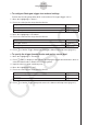
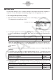

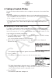
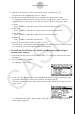
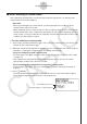
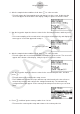
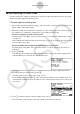

Table Of Contents
- Contenu
- Familiarisation — A lire en premier!
- Chapitre 1 Opérations de base
- Chapitre 2 Calculs manuels
- 1. Calculs de base
- 2. Fonctions spéciales
- 3. Spécification de l’unité d’angle et du format d’affichage
- 4. Calculs de fonctions
- 5. Calculs numériques
- 6. Calculs avec nombres complexes
- 7. Calculs binaire, octal, décimal et hexadécimal avec entiers
- 8. Calculs matriciels
- 9. Calculs vectoriels
- 10. Calculs de conversion métrique
- Chapitre 3 Listes
- Chapitre 4 Calcul d’équations
- Chapitre 5 Représentation graphique de fonctions
- 1. Exemples de graphes
- 2. Contrôle des paramètres apparaissant sur un écran graphique
- 3. Tracé d’un graphe
- 4. Stockage d’un graphe dans la mémoire d’images
- 5. Tracé de deux graphes sur le même écran
- 6. Représentation graphique manuelle
- 7. Utilisation de tables
- 8. Représentation graphique dynamique
- 9. Représentation graphique d’une formule de récurrence
- 10. Tracé du graphe d’une section conique
- 11. Changement de l’aspect d’un graphe
- 12. Analyse de fonctions
- Chapitre 6 Graphes et calculs statistiques
- 1. Avant d’effectuer des calculs statistiques
- 2. Calcul et représentation graphique de données statistiques à variable unique
- 3. Calcul et représentation graphique de données statistiques à variable double
- 4. Exécution de calculs statistiques
- 5. Tests
- 6. Intervalle de confiance
- 7. Lois de probabilité
- 8. Termes des tests d’entrée et sortie, intervalle de confiance et loi de probabilité
- 9. Formule statistique
- Chapitre 7 Calculs financiers
- 1. Avant d’effectuer des calculs financiers
- 2. Intérêt simple
- 3. Intérêt composé
- 4. Cash-flow (Évaluation d’investissement)
- 5. Amortissement
- 6. Conversion de taux d’intérêt
- 7. Coût, prix de vente, marge
- 8. Calculs de jours/date
- 9. Dépréciation
- 10. Calculs d’obligations
- 11. Calculs financiers en utilisant des fonctions
- Chapitre 8 Programmation
- 1. Étapes élémentaires de la programmation
- 2. Touches de fonction du mode PROGR (ou PRGM)
- 3. Édition du contenu d’un programme
- 4. Gestion de fichiers
- 5. Guide des commandes
- 6. Utilisation des fonctions de la calculatrice dans un programme
- 7. Liste des commandes du mode PROGR (ou PRGM)
- 8. Tableau de conversion des commandes spéciales de la calculatrice scientifique CASIO <=> Texte
- 9. Bibliothèque de programmes
- Chapitre 9 Feuille de Calcul
- Chapitre 10 L’eActivity
- Chapitre 11 Gestionnaire de la mémoire
- Chapitre 12 Menu de réglages du système
- Chapitre 13 Communication de données
- Chapitre 14 PYTHON
- 1. Aperçu du mode PYTHON
- 2. Menu de fonctions de PYTHON
- 3. Saisie de texte et de commandes
- 4. Utilisation du SHELL
- 5. Utilisation des fonctions de tracé (module casioplot)
- 6. Modification d’un fichier py
- 7. Gestion de dossiers (recherche et suppression de fichiers)
- 8. Compatibilité de fichier
- 9. Exemples de scripts
- Chapitre 15 Probabilités
- Appendice
- Mode Examen
- E-CON3 Application (English) (GRAPH35+ E II)
- 1 E-CON3 Overview
- 2 Using the Setup Wizard
- 3 Using Advanced Setup
- 4 Using a Custom Probe
- 5 Using the MULTIMETER Mode
- 6 Using Setup Memory
- 7 Using Program Converter
- 8 Starting a Sampling Operation
- 9 Using Sample Data Memory
- 10 Using the Graph Analysis Tools to Graph Data
- 11 Graph Analysis Tool Graph Screen Operations
- 12 Calling E-CON3 Functions from an eActivity

5. Input up to 18 characters for the custom probe name, and then press E.
• This will cause the highlighting to move to “Slope”.
6. Use the function keys described below to configure the custom probe setup.
• To change the setting of an item, first use the f and c cursor keys to move the
highlighting to the item. Next, use the function keys to select the setting you want.
(1) Slope
Press 1(EDIT) to input the slope for the linear interpolation formula.
(2) Intercept
Press 1(EDIT) to input the intercept for the linear interpolation formula.
(3) Unit Name
Press 1(EDIT) to input up to eight characters for the unit name.
(4) Warm-up
Press 1(EDIT) to input the warm-up time.
7. Press w and then input a memory number (1 to 99).
• This saves the custom probe setup and returns to the Custom Probe List, which should
now contain the new custom probe setup you configured.
u
To recall the specifications of a Vernier or CMA sensor and configure
custom probe settings
1. Perform the first two steps of the procedure under “To configure a custom probe setup”
on page 4-1.
2. Press 4(VRNR) or 5(CMA).
• This displays a sensor list.
3. Use the f and c keys to move the highlighting to the sensor whose setting you want
to use as the basis of the custom probe settings, and then press w.
• The name and specifications of the sensor you select will appear on the custom probe
setup screen.
• To complete this procedure, perform steps 4 through 7 under “To configure a custom
probe setup” (page 4-1).
4-2
Using a Custom Probe