
User Manual
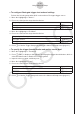
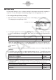
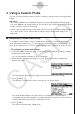
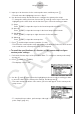

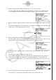

Table Of Contents
- Contenu
- Familiarisation — A lire en premier!
- Chapitre 1 Opérations de base
- Chapitre 2 Calculs manuels
- 1. Calculs de base
- 2. Fonctions spéciales
- 3. Spécification de l’unité d’angle et du format d’affichage
- 4. Calculs de fonctions
- 5. Calculs numériques
- 6. Calculs avec nombres complexes
- 7. Calculs binaire, octal, décimal et hexadécimal avec entiers
- 8. Calculs matriciels
- 9. Calculs vectoriels
- 10. Calculs de conversion métrique
- Chapitre 3 Listes
- Chapitre 4 Calcul d’équations
- Chapitre 5 Représentation graphique de fonctions
- 1. Exemples de graphes
- 2. Contrôle des paramètres apparaissant sur un écran graphique
- 3. Tracé d’un graphe
- 4. Stockage d’un graphe dans la mémoire d’images
- 5. Tracé de deux graphes sur le même écran
- 6. Représentation graphique manuelle
- 7. Utilisation de tables
- 8. Représentation graphique dynamique
- 9. Représentation graphique d’une formule de récurrence
- 10. Tracé du graphe d’une section conique
- 11. Changement de l’aspect d’un graphe
- 12. Analyse de fonctions
- Chapitre 6 Graphes et calculs statistiques
- 1. Avant d’effectuer des calculs statistiques
- 2. Calcul et représentation graphique de données statistiques à variable unique
- 3. Calcul et représentation graphique de données statistiques à variable double
- 4. Exécution de calculs statistiques
- 5. Tests
- 6. Intervalle de confiance
- 7. Lois de probabilité
- 8. Termes des tests d’entrée et sortie, intervalle de confiance et loi de probabilité
- 9. Formule statistique
- Chapitre 7 Calculs financiers (TVM)
- 1. Avant d’effectuer des calculs financiers
- 2. Intérêt simple
- 3. Intérêt composé
- 4. Cash-flow (Évaluation d’investissement)
- 5. Amortissement
- 6. Conversion de taux d’intérêt
- 7. Coût, prix de vente, marge
- 8. Calculs de jours/date
- 9. Dépréciation
- 10. Calculs d’obligations
- 11. Calculs financiers en utilisant des fonctions
- Chapitre 8 Programmation
- 1. Étapes élémentaires de la programmation
- 2. Touches de fonction du mode PRGM
- 3. Édition du contenu d’un programme
- 4. Gestion de fichiers
- 5. Guide des commandes
- 6. Utilisation des fonctions de la calculatrice dans un programme
- 7. Liste des commandes du mode PRGM
- 8. Tableau de conversion des commandes spéciales de la calculatrice scientifique CASIO <=> Texte
- 9. Bibliothèque de programmes
- Chapitre 9 Feuille de Calcul
- Chapitre 10 L’eActivity
- Chapitre 11 Gestionnaire de la mémoire
- Chapitre 12 Menu de réglages du système
- Chapitre 13 Communication de données
- Chapitre 14 PYTHON
- 1. Aperçu du mode PYTHON
- 2. Menu de fonctions de PYTHON
- 3. Saisie de texte et de commandes
- 4. Utilisation du SHELL
- 5. Utilisation des fonctions de tracé (module casioplot)
- 6. Modification d’un fichier py
- 7. Gestion de dossiers (recherche et suppression de fichiers)
- 8. Compatibilité de fichier
- 9. Exemples de scripts
- Chapitre 15 Distribution
- Appendice
- Mode Examen
- E-CON3 Application (English) (GRAPH35+ E II)
- 1 E-CON3 Overview
- 2 Using the Setup Wizard
- 3 Using Advanced Setup
- 4 Using a Custom Probe
- 5 Using the MULTIMETER Mode
- 6 Using Setup Memory
- 7 Using Program Converter
- 8 Starting a Sampling Operation
- 9 Using Sample Data Memory
- 10 Using the Graph Analysis Tools to Graph Data
- 11 Graph Analysis Tool Graph Screen Operations
- 12 Calling E-CON3 Functions from an eActivity

4 Using a Custom Probe
You can use the procedures in this section to configure a custom probe for use with a Data
Logger.
Important!
• The sensors (CASIO, Vernier, CMA) that appear on the list during Channel Setup (page
3-3) are E-CON3 mode standard sensors. If you want to use a sensor that is not included in
the list, configure custom probe settings.
• A sensor with an output voltage in the range of 0 to 5 volts can be configured with E-CON3
as a custom probe. Use of sensors with an output voltage outside of this range is not
supported.
k Configuring a Custom Probe Setup
To configure a custom probe setup, you must input values for the constants of the fixed
linear interpolation formula ( ax + b ). The required constants are slope ( a ) and intercept ( b ). x
in the above expression ( ax + b ) is the sampled voltage value (sampling range: 0 to 5 volts).
u
To configure a custom probe setup
1. From the E-CON3 main menu (page 1-1), press 1(SET) and then c(ADV) to display
the Advanced Setup menu.
• See “3 Using Advanced Setup” for more information.
2. On the Advanced Setup menu (page 3-1), press f(Custom Probe) to display the
Custom Probe List.
• The message “No Custom Probe” appears if the Custom Probe List is empty.
3. Press 1(NEW).
• This displays a custom probe setup screen like the one shown below.
• The initial default setting for the probe name is “Voltage(6pin)”. The first step for
configuring custom probe settings is to change this name to another one. If you want to
leave the default name the way it is, skip steps 4 and 5.
4. Press 1(EDIT).
• This enters the probe name editing mode.
4-1
Using a Custom Probe