
User Manual
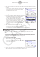
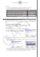
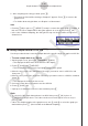
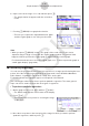
Table Of Contents
- Sisältö
- Tutustuminen — Aloita tästä!
- Luku 1 Perustoiminta
- Luku 2 Manuaaliset laskutoimitukset
- 1. Peruslaskutoimitukset
- 2. Erikoisfunktiot
- 3. Kulmatilan ja näyttömuodon määrittäminen
- 4. Funktiolaskutoimitukset
- 5. Numeeriset laskutoimitukset
- 6. Kompleksilukulaskutoimitukset
- 7. Kokonaislukujen binääri-, oktaali-, desimaali- ja heksadesimaalilaskutoimitukset
- 8. Matriisilaskutoimitukset
- 9. Vektorilaskutoimitukset
- 10. Yksikkömuunnoslaskutoimitukset
- Luku 3 Listatoiminto
- Luku 4 Yhtälölaskutoimitukset
- Luku 5 Kuvaajat
- 1. Kuvaajaesimerkkejä
- 2. Kuvaajanäytön näkymän määrittäminen
- 3. Kuvaajan piirtäminen
- 4. Kuvaajanäytön sisällön tallentaminen ja palauttaminen
- 5. Kahden kuvaajan piirtäminen samaan näyttöön
- 6. Kuvaajien piirtäminen manuaalisesti
- 7. Taulukoiden käyttäminen
- 8. Kuvaajan muokkaaminen
- 9. Kuvaajien dynaaminen piirtäminen
- 10. Rekursiokaavan kuvaajien piirtäminen
- 11. Kartioleikkausten piirtäminen
- 12. Pisteiden, viivojen ja tekstin piirtäminen kuvaajanäyttöön (Sketch)
- 13. Funktioanalyysi
- Luku 6 Tilastolliset kuvaajat ja laskutoimitukset
- 1. Ennen tilastollisten laskutoimitusten suorittamista
- 2. Yhden muuttujan tilastotietojen laskeminen ja niiden kuvaajat
- 3. Kahden muuttujan tilastotietojen laskeminen ja niiden kuvaajat (käyrän sovitus)
- 4. Tilastolaskutoimitusten suorittaminen
- 5. Testit
- 6. Luottamusväli
- 7. Jakauma
- 8. Testien syöte- ja tulostermit, luottamusväli ja jakauma
- 9. Tilastolliset kaavat
- Luku 7 Talouslaskutoimitukset
- Luku 8 Ohjelmointi
- Luku 9 Taulukkolaskenta
- Luku 10 eActivity
- Luku 11 Muistinhallinta
- Luku 12 Järjestelmänhallinta
- Luku 13 Tietoliikenne
- Luku 14 Geometria
- Luku 15 Picture Plot -toiminto
- Luku 16 3D-kuvaajatoiminto
- Luku 17 Python (vain fx-CG50, fx-CG50 AU)
- Luku 18 Jakauma (vain fx-CG50, fx-CG50 AU)
- Liite
- Koemoodit
- E-CON4 Application (English)
- 1. E-CON4 Mode Overview
- 2. Sampling Screen
- 3. Auto Sensor Detection (CLAB Only)
- 4. Selecting a Sensor
- 5. Configuring the Sampling Setup
- 6. Performing Auto Sensor Calibration and Zero Adjustment
- 7. Using a Custom Probe
- 8. Using Setup Memory
- 9. Starting a Sampling Operation
- 10. Using Sample Data Memory
- 11. Using the Graph Analysis Tools to Graph Data
- 12. Graph Analysis Tool Graph Screen Operations
- 13. Calling E-CON4 Functions from an eActivity

ε-45
Graph Analysis Tool Graph Screen Operations
6. Input a value in the range of 1 to 10, and then press w.
• The graph relation list appears with the calculation
result.
7. Pressing 6(DRAW) here graphs the function.
• This lets you compare the expanded function graph
and the original graph to see if they are the same.
Note
• When you press 6(DRAW) in step 7, the graph of the result of the Fourier series
expansion may not align correctly with the original graph on which it is overlaid. If this
happens, shift the position the original graph to align it with the overlaid graph.
For information about how to move the original graph, see “To move a particular graph on
a multi-graph display” (page
ε-48).
k Performing Regression
You can use the procedure below to perform regression for a range specified using the trace
pointer. All of the following regression types are supported: Linear, Med-Med, Quadratic,
Cubic, Quartic, Logarithmic, Exponential, Power, Sine, and Logistic.
For details about these regression types, see Chapter 6 of this manual.
The following procedure shows how to perform quadratic regression. The same general
steps can also be used to perform the other types of regression.
• To perform quadratic regression
1. On the graph screen, press K, and then 4(CALC).
• The CALC menu appears at the bottom of the display.
2. Press 5(X
2
).
• This displays the trace pointer for selecting the range
on the graph.
3. Move the trace pointer to the start point of the range for which you want to perform
quadratic regression, and then press w.