
User Manual
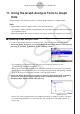
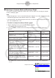


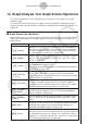

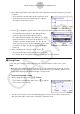
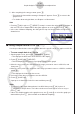
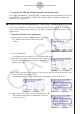
Table Of Contents
- Inhalt
- Einführung – Bitte dieses Kapitel zuerst durchlesen
- Kapitel 1 Grundlegende Operation
- Kapitel 2 Manuelle Berechnungen
- 1. Grundrechenarten
- 2. Spezielle Taschenrechnerfunktionen
- 3. Festlegung des Winkelmodus und des Anzeigeformats (SET UP)
- 4. Funktionsberechnungen
- 5. Numerische Berechnungen
- 6. Rechnen mit komplexen Zahlen
- 7. Rechnen mit (ganzen) Binär-, Oktal-, Dezimal- und Hexadezimalzahlen
- 8. Matrizenrechnung
- 9. Vektorrechnung
- 10. Umrechnen von Maßeinheiten
- Kapitel 3 Listenoperationen
- Kapitel 4 Lösung von Gleichungen
- Kapitel 5 Grafische Darstellungen
- 1. Graphenbeispiele
- 2. Voreinstellungen verschiedenster Art für eine optimale Graphenanzeige
- 3. Zeichnen eines Graphen
- 4. Speichern und Aufrufen von Inhalten des Graphenbildschirms
- 5. Zeichnen von zwei Graphen im gleichen Display
- 6. Manuelle grafische Darstellung
- 7. Verwendung von Wertetabellen
- 8. Ändern eines Graphen
- 9. Dynamischer Graph (Graphanimation einer Kurvenschar)
- 10. Grafische Darstellung von Rekursionsformeln
- 11. Grafische Darstellung eines Kegelschnitts
- 12. Zeichnen von Punkten, Linien und Text im Graphenbildschirm (Sketch)
- 13. Funktionsanalyse (Kurvendiskussion)
- Kapitel 6 Statistische Grafiken und Berechnungen
- 1. Vor dem Ausführen statistischer Berechnungen
- 2. Berechnungen und grafische Darstellungen mit einer eindimensionalen Stichprobe
- 3. Berechnungen und grafische Darstellungen mit einer zweidimensionalen Stichprobe (Ausgleichungsrechnung)
- 4. Ausführung statistischer Berechnungen und Ermittlung von Wahrscheinlichkeiten
- 5. Tests
- 6. Konfidenzintervall
- 7. Wahrscheinlichkeitsverteilungen
- 8. Ein- und Ausgabebedingungen für statistische Testverfahren, Konfidenzintervalle und Wahrscheinlichkeitsverteilungen
- 9. Statistikformeln
- Kapitel 7 Finanzmathematik
- 1. Vor dem Ausführen finanzmathematischer Berechnungen
- 2. Einfache Kapitalverzinsung
- 3. Kapitalverzinsung mit Zinseszins
- 4. Cashflow-Berechnungen (Investitionsrechnung)
- 5. Tilgungsberechnungen (Amortisation)
- 6. Zinssatz-Umrechnung
- 7. Herstellungskosten, Verkaufspreis, Gewinnspanne
- 8. Tages/Datums-Berechnungen
- 9. Abschreibung
- 10. Anleihenberechnungen
- 11. Finanzmathematik unter Verwendung von Funktionen
- Kapitel 8 Programmierung
- 1. Grundlegende Programmierschritte
- 2. Program-Menü-Funktionstasten
- 3. Editieren von Programminhalten
- 4. Programmverwaltung
- 5. Befehlsreferenz
- 6. Verwendung von Rechnerbefehlen in Programmen
- 7. Program-Menü-Befehlsliste
- 8. CASIO-Rechner für wissenschaftliche Funktionswertberechnungen Spezielle Befehle <=> Textkonvertierungstabelle
- 9. Programmbibliothek
- Kapitel 9 Tabellenkalkulation
- 1. Grundlagen der Tabellenkalkulation und das Funktionsmenü
- 2. Grundlegende Operationen in der Tabellenkalkulation
- 3. Verwenden spezieller Befehle des Spreadsheet-Menüs
- 4. Bedingte Formatierung
- 5. Zeichnen von statistischen Graphen sowie Durchführen von statistischen Berechnungen und Regressionsanalysen
- 6. Speicher des Spreadsheet-Menüs
- Kapitel 10 eActivity
- Kapitel 11 Speicherverwalter
- Kapitel 12 Systemverwalter
- Kapitel 13 Datentransfer
- Kapitel 14 Geometrie
- Kapitel 15 Picture Plot
- Kapitel 16 3D Graph-Funktion
- Kapitel 17 Python (nur fx-CG50, fx-CG50 AU)
- Kapitel 18 Verteilung (nur fx-CG50, fx-CG50 AU)
- Anhang
- Prüfungsmodi
- E-CON4 Application (English)
- 1. E-CON4 Mode Overview
- 2. Sampling Screen
- 3. Auto Sensor Detection (CLAB Only)
- 4. Selecting a Sensor
- 5. Configuring the Sampling Setup
- 6. Performing Auto Sensor Calibration and Zero Adjustment
- 7. Using a Custom Probe
- 8. Using Setup Memory
- 9. Starting a Sampling Operation
- 10. Using Sample Data Memory
- 11. Using the Graph Analysis Tools to Graph Data
- 12. Graph Analysis Tool Graph Screen Operations
- 13. Calling E-CON4 Functions from an eActivity

ε-43
Graph Analysis Tool Graph Screen Operations
5. After everything is the way you want, press w.
• This saves the lists and the message “Complete!” appears. Press w to return to the
graph screen.
• For details about using list data, see Chapter 3 of this manual.
Note
• Pressing 1(All) in place of 2(SELECT) in step 2 converts the entire graph to list data. In
this case, the “Store Sample Data” dialog box appears as soon as you press 1(All).
• In the case of Manual Sampling, the dialog box in step 4 of the procedure will appear as
shown below.
k Saving Sample Data to a CSV File
Use the procedure below to save the sample data in the specific range of a graph to a CSV file.
• To save sample data to a CSV file
1. On the graph screen, press K2(MEMORY)2(CSV).
• This displays the CSV menu at the bottom of the display.
2. Press 1(SAVE
•
AS)2(SELECT).
• This will display a trace point for specifying a range on the graph.
3. Move the trace point to the start point of the range you want to save to a CSV file, and
then press w.
4. Move the trace point to the end point of the range you want to save to a CSV file, and then
press w.
• This displays the folder selection screen.
5. Select the folder where you want to save the CSV file.
6. Press 1(SAVE
•
AS).
7. Input up to 8 characters for the file name and then press w.
Note
• To select all of the graph data and save it as CSV data, press 1(All) in place of
2(SELECT) in step 2 above. The folder selection screen will appear as soon as you
press 1(All).
• If there are multiple graphs on the graph screen, use f and c to select the graph you
want and then press w. (Not included on the Manual Sampling)