
User Manual
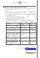

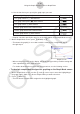


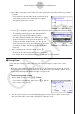
Table Of Contents
- Sisältö
- Tutustuminen — Aloita tästä!
- Luku 1 Perustoiminta
- Luku 2 Manuaaliset laskutoimitukset
- 1. Peruslaskutoimitukset
- 2. Erikoisfunktiot
- 3. Kulmatilan ja näyttömuodon määrittäminen
- 4. Funktiolaskutoimitukset
- 5. Numeeriset laskutoimitukset
- 6. Kompleksilukulaskutoimitukset
- 7. Kokonaislukujen binääri-, oktaali-, desimaali- ja heksadesimaalilaskutoimitukset
- 8. Matriisilaskutoimitukset
- 9. Vektorilaskutoimitukset
- 10. Yksikkömuunnoslaskutoimitukset
- Luku 3 Listatoiminto
- Luku 4 Yhtälölaskutoimitukset
- Luku 5 Kuvaajat
- 1. Kuvaajaesimerkkejä
- 2. Kuvaajanäytön näkymän määrittäminen
- 3. Kuvaajan piirtäminen
- 4. Kuvaajanäytön sisällön tallentaminen ja palauttaminen
- 5. Kahden kuvaajan piirtäminen samaan näyttöön
- 6. Kuvaajien piirtäminen manuaalisesti
- 7. Taulukoiden käyttäminen
- 8. Kuvaajan muokkaaminen
- 9. Kuvaajien dynaaminen piirtäminen
- 10. Rekursiokaavan kuvaajien piirtäminen
- 11. Kartioleikkausten piirtäminen
- 12. Pisteiden, viivojen ja tekstin piirtäminen kuvaajanäyttöön (Sketch)
- 13. Funktioanalyysi
- Luku 6 Tilastolliset kuvaajat ja laskutoimitukset
- 1. Ennen tilastollisten laskutoimitusten suorittamista
- 2. Yhden muuttujan tilastotietojen laskeminen ja niiden kuvaajat
- 3. Kahden muuttujan tilastotietojen laskeminen ja niiden kuvaajat (käyrän sovitus)
- 4. Tilastolaskutoimitusten suorittaminen
- 5. Testit
- 6. Luottamusväli
- 7. Jakauma
- 8. Testien syöte- ja tulostermit, luottamusväli ja jakauma
- 9. Tilastolliset kaavat
- Luku 7 Talouslaskutoimitukset
- Luku 8 Ohjelmointi
- Luku 9 Taulukkolaskenta
- Luku 10 eActivity
- Luku 11 Muistinhallinta
- Luku 12 Järjestelmänhallinta
- Luku 13 Tietoliikenne
- Luku 14 Geometria
- Luku 15 Picture Plot -toiminto
- Luku 16 3D-kuvaajatoiminto
- Luku 17 Python (vain fx-CG50, fx-CG50 AU)
- Luku 18 Jakauma (vain fx-CG50, fx-CG50 AU)
- Liite
- Koemoodit
- E-CON4 Application (English)
- 1. E-CON4 Mode Overview
- 2. Sampling Screen
- 3. Auto Sensor Detection (CLAB Only)
- 4. Selecting a Sensor
- 5. Configuring the Sampling Setup
- 6. Performing Auto Sensor Calibration and Zero Adjustment
- 7. Using a Custom Probe
- 8. Using Setup Memory
- 9. Starting a Sampling Operation
- 10. Using Sample Data Memory
- 11. Using the Graph Analysis Tools to Graph Data
- 12. Graph Analysis Tool Graph Screen Operations
- 13. Calling E-CON4 Functions from an eActivity
ε-36
Using the Graph Analysis Tools to Graph Data
k Selecting an Analysis Mode and Drawing a Graph
This section contains a detailed procedure that covers all steps from selecting an analysis
mode to drawing a graph.
Note
• Step 4 through step 7 are not essential and may be skipped, if you want. Skipping any step
automatically applies the initial default values for its settings.
• If you skip step 2, the default analysis mode is the one whose name is displayed in the top
line of the Graph Mode screen.
• To select an analysis mode and draw a graph
1. On the sampling screen, press 4(OTHER)1(GRAPH).
• This displays the Graph Mode screen.
2. Press 3(MODE), and then select the analysis mode you want from the menu that
appears.
To do this:
Perform this menu
operation:
To select this
mode:
Graph three sets of sampled data
simultaneously
[Norm] Graph Analysis
Graph sampled data along with its first
and second derivative graph
[diff] d/dt & d
2
/dt
2
Display the graphs of different sampled
data in upper and lower windows for
comparison
[COMPARE] → [GRAPH]
Compare Graph
Output sampled data from the speaker,
displaying graph of the raw data in
the upper window and the output
waveform in the lower window (EA-200
only)
[COMPARE] → [Sound]
Compare Sound
Display the graph of sampled data
in the upper window and its first
derivative graph in the lower window
[COMPARE] → [d/dt]
Compare d/dt
Display the graph of sampled data
in the upper window and its second
derivative graph in the lower window
[COMPARE] → [d
2
/dt
2
]
Compare d
2
/dt
2
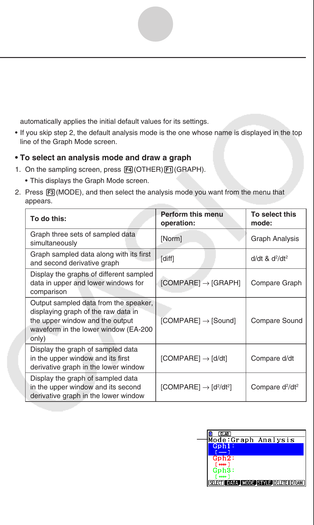
• The name of the currently selected mode appears in the top line of the Graph Mode
screen.
Analysis mode name