
User Manual
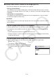
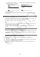

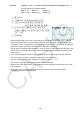
Table Of Contents
- Contents
- Getting Acquainted — Read This First!
- Chapter 1 Basic Operation
- Chapter 2 Manual Calculations
- 1. Basic Calculations
- 2. Special Functions
- 3. Specifying the Angle Unit and Display Format
- 4. Function Calculations
- 5. Numerical Calculations
- 6. Complex Number Calculations
- 7. Binary, Octal, Decimal, and Hexadecimal Calculations with Integers
- 8. Matrix Calculations
- 9. Vector Calculations
- 10. Metric Conversion Calculations
- Chapter 3 List Function
- Chapter 4 Equation Calculations
- Chapter 5 Graphing
- 1. Sample Graphs
- 2. Controlling What Appears on a Graph Screen
- 3. Drawing a Graph
- 4. Saving and Recalling Graph Screen Contents
- 5. Drawing Two Graphs on the Same Screen
- 6. Manual Graphing
- 7. Using Tables
- 8. Modifying a Graph
- 9. Dynamic Graphing
- 10. Graphing a Recursion Formula
- 11. Graphing a Conic Section
- 12. Drawing Dots, Lines, and Text on the Graph Screen (Sketch)
- 13. Function Analysis
- Chapter 6 Statistical Graphs and Calculations
- 1. Before Performing Statistical Calculations
- 2. Calculating and Graphing Single-Variable Statistical Data
- 3. Calculating and Graphing Paired-Variable Statistical Data (Curve Fitting)
- 4. Performing Statistical Calculations
- 5. Tests
- 6. Confidence Interval
- 7. Distribution
- 8. Input and Output Terms of Tests, Confidence Interval, and Distribution
- 9. Statistic Formula
- Chapter 7 Financial Calculation
- Chapter 8 Programming
- Chapter 9 Spreadsheet
- Chapter 10 eActivity
- Chapter 11 Memory Manager
- Chapter 12 System Manager
- Chapter 13 Data Communication
- Chapter 14 Geometry
- Chapter 15 Picture Plot
- Chapter 16 3D Graph Function
- Chapter 17 Python (fx-CG50, fx-CG50 AU only)
- Appendix
- Examination Mode
- E-CON4 Application
- 1. E-CON4 Mode Overview
- 2. Sampling Screen
- 3. Auto Sensor Detection (CLAB Only)
- 4. Selecting a Sensor
- 5. Configuring the Sampling Setup
- 6. Performing Auto Sensor Calibration and Zero Adjustment
- 7. Using a Custom Probe
- 8. Using Setup Memory
- 9. Starting a Sampling Operation
- 10. Using Sample Data Memory
- 11. Using the Graph Analysis Tools to Graph Data
- 12. Graph Analysis Tool Graph Screen Operations
- 13. Calling E-CON4 Functions from an eActivity
5-25
6. Manual Graphing
k Graphing in the Run-Matrix Mode
While the Linear input/output mode is selected, commands can be input directly in the Run-
Matrix mode to draw a graph.
You can select a function type for graphing by pressing !4(SKETCH)5(GRAPH) and
then selecting one of the function types shown below.
• {Y=}/{r=}/{Param}/{X=}/{G ·
dx} ... {rectangular coordinate}/{polar coordinate}/{parametric
function}/{X=f(y) rectangular coordinate}/{integration} graphing
• {Y>}/{Y<}/{Y≥}/{Y≤} ... Inequality {Y>
f(x)}/{Y<f(x)}/{Y≥f(x)}/{Y≤f(x)} graphing
• {X>}/{X<}/{X≥}/{X≤} ... Inequality {X>
f(y)}/{X<f(y)}/{X≥f(y)}/{X≤f(y)} graphing
• Graphing with Rectangular Coordinates
1. From the Main Menu, enter the Run-Matrix mode.
2. On the Setup screen, change “Input/Output” setting to “Linear”.
3. Configure V-Window settings.
4. Input the commands for drawing the rectangular coordinate graph.
5. Input the function.
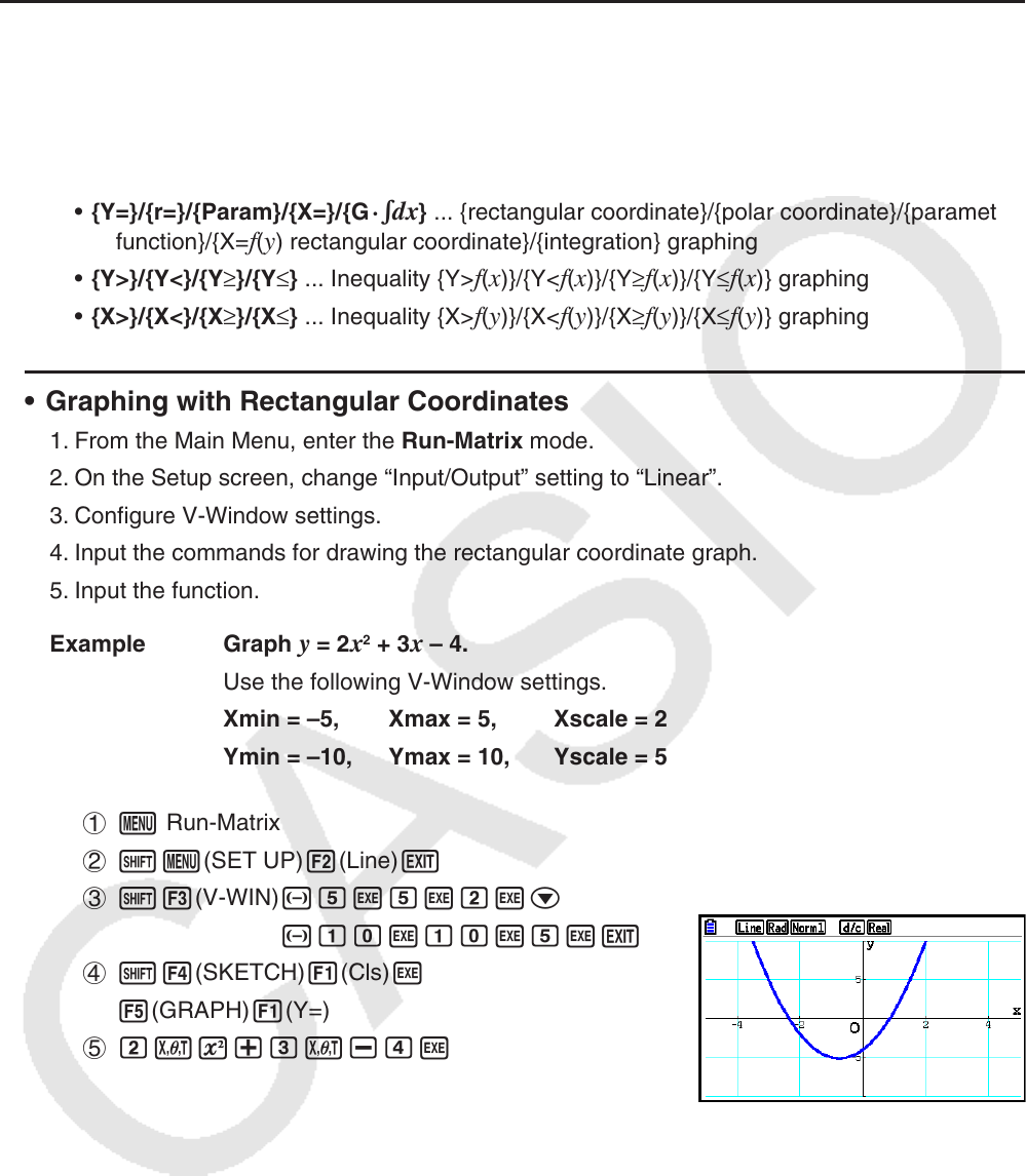
Example Graph
y = 2x
2
+ 3x – 4.
Use the following V-Window settings.
Xmin = –5, Xmax = 5, Xscale = 2
Ymin = –10, Ymax = 10, Yscale = 5
1 m Run-Matrix
2 !m(SET UP)2(Line)J
3 !3(V-WIN) -fwfwcwc
-bawbawfwJ
4 !4(SKETCH)1(Cls)w
5(GRAPH)1(Y=)
5 cvx+dv-ew