
User Manual
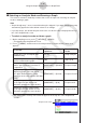
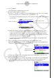
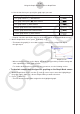
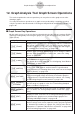
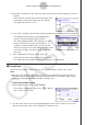
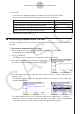
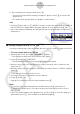
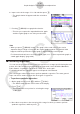
Table Of Contents
- Inhoud
- Eerste kennismaking — Lees dit eerst!
- Hoofdstuk 1 Basisbewerking
- Hoofdstuk 2 Handmatige berekeningen
- 1. Basisberekeningen
- 2. Speciale functies
- 3. De hoekeenheid en weergave van getallen instellen
- 4. Functieberekeningen
- 5. Numerieke berekeningen
- 6. Rekenen met complexe getallen
- 7. Berekeningen met gehele getallen in het twee-, acht-, tien- en zestientallige talstelsel
- 8. Matrixberekeningen
- 9. Vectorberekeningen
- 10. Metrieke omzetting
- Hoofdstuk 3 Lijsten
- Hoofdstuk 4 Vergelijkingen berekenen
- Hoofdstuk 5 Grafieken tekenen
- 1. Voorbeeldgrafieken
- 2. Bepalen wat wordt weergegeven in een grafiekscherm
- 3. Een grafiek tekenen
- 4. Inhoud van het grafiekscherm opslaan en oproepen
- 5. Twee grafieken in hetzelfde scherm tekenen
- 6. Handmatig tekenen
- 7. Tabellen gebruiken
- 8. Een grafiek wijzigen
- 9. Dynamische grafieken tekenen
- 10. Een grafiek tekenen op basis van een recursieformule
- 11. Grafieken van kegelsneden tekenen
- 12. Punten, lijnen en tekst tekenen in het grafiekscherm (Sketch)
- 13. Functieanalyse
- Hoofdstuk 6 Statistische grafieken en berekeningen
- 1. Voor u met statistische berekeningen begint
- 2. Grafieken en berekeningen voor statistische gegevens met één variabele
- 3. Grafieken en berekeningen voor statistische gegevens met twee variabelen (Aanpassing kromme)
- 4. Statistische berekeningen uitvoeren
- 5. Testen
- 6. Betrouwbaarheidsinterval
- 7. Kansverdelingsfuncties
- 8. Invoer- en uitvoertermen van testen, betrouwbaarheidsinterval en kansverdelingsfuncties
- 9. Statistische formule
- Hoofdstuk 7 Financiële berekeningen
- 1. Voor u met financiële berekeningen begint
- 2. Een enkelvoudige interest berekenen
- 3. Een samengestelde interest berekenen
- 4. Evaluatie van een investering (cashflow)
- 5. Afschrijving van een lening
- 6. Omzetting van nominale rentevoet naar reële rentevoet
- 7. Berekening van kosten, verkoopprijs en winstmarge
- 8. Dag- en datumberekeningen
- 9. Devaluatie
- 10. Obligatieberekeningen
- 11. Financiële berekeningen met gebruik van functies
- Hoofdstuk 8 Programmeren
- 1. Basishandelingen voor het programmeren
- 2. Functietoetsen in de modus Program
- 3. De programma-inhoud wijzigen
- 4. Bestandsbeheer
- 5. Overzicht van de opdrachten
- 6. Rekenmachinefuncties gebruiken bij het programmeren
- 7. Lijst met opdrachten in de modus Program
- 8. Wetenschappelijke CASIO-specifieke functieopdrachten <=> Tekstconversietabel
- 9. Programmablad
- Hoofdstuk 9 Spreadsheet
- Hoofdstuk 10 eActivity
- Hoofdstuk 11 Geheugenbeheer
- Hoofdstuk 12 Systeembeheer
- Hoofdstuk 13 Gegevenscommunicatie
- Hoofdstuk 14 Geometry
- Hoofdstuk 15 Picture Plot
- Hoofdstuk 16 3D-grafiek functie
- Hoofdstuk 17 Python (alleen fx-CG50, fx-CG50 AU)
- Hoofdstuk 18 Kansverdeling (alleen fx-CG50, fx-CG50 AU)
- Bijlage
- Examenmodi
- E-CON4 Application (English)
- 1. E-CON4 Mode Overview
- 2. Sampling Screen
- 3. Auto Sensor Detection (CLAB Only)
- 4. Selecting a Sensor
- 5. Configuring the Sampling Setup
- 6. Performing Auto Sensor Calibration and Zero Adjustment
- 7. Using a Custom Probe
- 8. Using Setup Memory
- 9. Starting a Sampling Operation
- 10. Using Sample Data Memory
- 11. Using the Graph Analysis Tools to Graph Data
- 12. Graph Analysis Tool Graph Screen Operations
- 13. Calling E-CON4 Functions from an eActivity

ε-45
Graph Analysis Tool Graph Screen Operations
6. Input a value in the range of 1 to 10, and then press w.
• The graph relation list appears with the calculation
result.
7. Pressing 6(DRAW) here graphs the function.
• This lets you compare the expanded function graph
and the original graph to see if they are the same.
Note
• When you press 6(DRAW) in step 7, the graph of the result of the Fourier series
expansion may not align correctly with the original graph on which it is overlaid. If this
happens, shift the position the original graph to align it with the overlaid graph.
For information about how to move the original graph, see “To move a particular graph on
a multi-graph display” (page
ε-48).
k Performing Regression
You can use the procedure below to perform regression for a range specified using the trace
pointer. All of the following regression types are supported: Linear, Med-Med, Quadratic,
Cubic, Quartic, Logarithmic, Exponential, Power, Sine, and Logistic.
For details about these regression types, see Chapter 6 of this manual.
The following procedure shows how to perform quadratic regression. The same general
steps can also be used to perform the other types of regression.
• To perform quadratic regression
1. On the graph screen, press K, and then 4(CALC).
• The CALC menu appears at the bottom of the display.
2. Press 5(X
2
).
• This displays the trace pointer for selecting the range
on the graph.
3. Move the trace pointer to the start point of the range for which you want to perform
quadratic regression, and then press w.