
User Manual
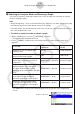
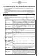
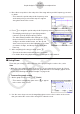
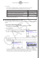
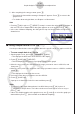

Table Of Contents
- Innhold
- Bli kjent – Les dette først!
- Kapittel 1 Grunnleggende bruk
- Kapittel 2 Manuelle beregninger
- 1. Grunnleggende beregninger
- 2. Spesialfunksjoner
- 3. Angi vinkelenhet og displayformat
- 4. Funksjonsberegninger
- 5. Numeriske beregninger
- 6. Beregninger med komplekse tall
- 7. Binære, oktale, desimale og heksadesimale heltallsberegninger
- 8. Matriseberegninger
- 9. Vektorberegninger
- 10. Metriske omformingsberegninger
- Kapittel 3 Listefunksjon
- Kapittel 4 Likningsberegninger
- Kapittel 5 Graftegning
- 1. Eksempelgrafer
- 2. Bestemme hva som skal vises på et grafskjermbilde
- 3. Tegne en graf
- 4. Lagre og hente frem innholdet av grafskjermbildet
- 5. Tegne to grafer på samme skjerm
- 6. Manuell graftegning
- 7. Bruke tabeller
- 8. Endre en graf
- 9. Dynamisk grafskriving
- 10. Tegne graf for en rekursjonsformel
- 11. Tegne kjeglesnitt som graf
- 12. Tegning av punkter, linjer og tekst på grafskjermen (Skisse)
- 13. Funksjonsanalyse
- Kapittel 6 Statistiske grafer og beregninger
- 1. Før du utfører statistiske beregninger
- 2. Beregne og tegne grafer for statistiske data med én variabel
- 3. Beregne og tegne grafer for statistiske data med parvise variabler (kurve montering)
- 4. Utføre statistiske beregninger
- 5. Tester
- 6. Konfidensintervall
- 7. Distribusjon
- 8. Inntastings- og utdataledd for tester, konfidensintervall og distribusjon
- 9. Statistisk formel
- Kapittel 7 Økonomiske beregninger
- 1. Før du utfører økonomiske beregninger
- 2. Vanlig rente
- 3. Rentes rente
- 4. Kontantstrøm (investeringsvurdering)
- 5. Amortisering
- 6. Omregning av rentefot
- 7. Kostnad, salgspris, fortjenestemargin
- 8. Dag-/datoberegninger
- 9. Avskrivning
- 10. Obligasjonsberegninger
- 11. Økonomiske beregninger ved hjelp av funksjoner
- Kapittel 8 Programmering
- 1. Grunnleggende programmeringstrinn
- 2. Funksjonstaster for Program-modus
- 3. Redigere programinnhold
- 4. Filbehandling
- 5. Kommandoreferanse
- 6. Bruke kalkulatorfunksjoner i programmer
- 7. Kommandolisten i Program-modus
- 8. CASIO-kalkulator med vitenskapelige funksjoner Spesialkommandoer <=> Tekstkonverteringstabell
- 9. Programbibliotek
- Kapittel 9 Regneark
- Kapittel 10 eActivity
- Kapittel 11 Minnehåndtering
- Kapittel 12 Systemhåndtering
- Kapittel 13 Datakommunikasjon
- Kapittel 14 Geometri
- Kapittel 15 Picture Plot
- Kapittel 16 3D-graffunksjon
- Kapittel 17 Python (kun fx-CG50, fx-CG50 AU)
- Kapittel 18 Distribusjon (kun fx-CG50, fx-CG50 AU)
- Vedlegg
- Examination Modes
- E-CON4 Application (English)
- 1. E-CON4 Mode Overview
- 2. Sampling Screen
- 3. Auto Sensor Detection (CLAB Only)
- 4. Selecting a Sensor
- 5. Configuring the Sampling Setup
- 6. Performing Auto Sensor Calibration and Zero Adjustment
- 7. Using a Custom Probe
- 8. Using Setup Memory
- 9. Starting a Sampling Operation
- 10. Using Sample Data Memory
- 11. Using the Graph Analysis Tools to Graph Data
- 12. Graph Analysis Tool Graph Screen Operations
- 13. Calling E-CON4 Functions from an eActivity

ε-39
Graph Analysis Tool Graph Screen Operations
12.
Graph Analysis Tool Graph Screen Operations
This section explains the various operations you can perform on the graph screen after
drawing a graph.
You can perform these operations on a graph screen produced by a sampling operation,
or by the operation described under “Selecting an Analysis Mode and Drawing a Graph” on
page
ε-36.
k Graph Screen Key Operations
On the graph screen, you can use the keys described in the table below to analyze (CALC)
graphs by reading data points along the graph (Trace) and enlarging specific parts of the
graph (Zoom).
Key Operation Description
!1(TRACE)
Displays a trace pointer on the graph along with the coordinates of
the current cursor location. Trace can also be used to obtain the
periodic frequency of a specific range on the graph and assign it
to a variable. See “Using Trace” on page
ε-40.
!2(ZOOM)
Starts a zoom operation, which you can use to enlarge or reduce
the size of the graph along the
x-axis or the y-axis. See “Using
Zoom” on page ε-41.
!3(V-WIN)
Displays a function menu of special View Window commands for
the E-CON4 mode graph screen.
For details about each command, see “Configuring View Window
Parameters” on page
ε-49.
!4(SKETCH)
Displays a menu that contains the following commands: Cls, Plot,
F-Line, Text, PEN, Vertical, and Horizontal. For details about
each command, see “Drawing Dots, Lines, and Text on the Graph
Screen (Sketch)” on
page 5-52.
K1(PICTURE)
Saves the currently displayed graph as a graphic image. You can
recall a saved graph image and overlay it on another graph to
compare them. For details about these procedures, see “Saving
and Recalling Graph Screen Contents” on page 5-20.
K2(MEMORY)
1(LISTMEM)
Displays a menu of functions for saving the sample values in a
specific range of a graph to a list. See “Transforming Sampled
Data to List Data” on page ε-42.
K2(MEMORY)
2(CSV)
Saves the sample data in the specific range of a graph to a CSV
file. For details, see “Saving Sample Data to a CSV File” (page
ε-43).
K3(EDIT)
Displays a menu of functions for zooming and editing a particular
graph when the graph screen contains multiple graphs. See
“Working with Multiple Graphs” on page
ε-46.
K4(CALC)
Displays a menu that lets you transform a sample result graph to a
function using Fourier series expansion, and to perform regression
to determine the tendency of a graph. See “Using Fourier Series
Expansion to Transform a Waveform to a Function” on page
ε-44,
and “Performing Regression” on page ε-45.