
User Manual


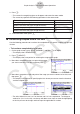


Table Of Contents
- Inhalt
- Einführung – Bitte dieses Kapitel zuerst durchlesen
- Kapitel 1 Grundlegende Operation
- Kapitel 2 Manuelle Berechnungen
- 1. Grundrechenarten
- 2. Spezielle Taschenrechnerfunktionen
- 3. Festlegung des Winkelmodus und des Anzeigeformats (SET UP)
- 4. Funktionsberechnungen
- 5. Numerische Berechnungen
- 6. Rechnen mit komplexen Zahlen
- 7. Rechnen mit (ganzen) Binär-, Oktal-, Dezimal- und Hexadezimalzahlen
- 8. Matrizenrechnung
- 9. Vektorrechnung
- 10. Umrechnen von Maßeinheiten
- Kapitel 3 Listenoperationen
- Kapitel 4 Lösung von Gleichungen
- Kapitel 5 Grafische Darstellungen
- 1. Graphenbeispiele
- 2. Voreinstellungen verschiedenster Art für eine optimale Graphenanzeige
- 3. Zeichnen eines Graphen
- 4. Speichern und Aufrufen von Inhalten des Graphenbildschirms
- 5. Zeichnen von zwei Graphen im gleichen Display
- 6. Manuelle grafische Darstellung
- 7. Verwendung von Wertetabellen
- 8. Ändern eines Graphen
- 9. Dynamischer Graph (Graphanimation einer Kurvenschar)
- 10. Grafische Darstellung von Rekursionsformeln
- 11. Grafische Darstellung eines Kegelschnitts
- 12. Zeichnen von Punkten, Linien und Text im Graphenbildschirm (Sketch)
- 13. Funktionsanalyse (Kurvendiskussion)
- Kapitel 6 Statistische Grafiken und Berechnungen
- 1. Vor dem Ausführen statistischer Berechnungen
- 2. Berechnungen und grafische Darstellungen mit einer eindimensionalen Stichprobe
- 3. Berechnungen und grafische Darstellungen mit einer zweidimensionalen Stichprobe (Ausgleichungsrechnung)
- 4. Ausführung statistischer Berechnungen und Ermittlung von Wahrscheinlichkeiten
- 5. Tests
- 6. Konfidenzintervall
- 7. Wahrscheinlichkeitsverteilungen
- 8. Ein- und Ausgabebedingungen für statistische Testverfahren, Konfidenzintervalle und Wahrscheinlichkeitsverteilungen
- 9. Statistikformeln
- Kapitel 7 Finanzmathematik
- 1. Vor dem Ausführen finanzmathematischer Berechnungen
- 2. Einfache Kapitalverzinsung
- 3. Kapitalverzinsung mit Zinseszins
- 4. Cashflow-Berechnungen (Investitionsrechnung)
- 5. Tilgungsberechnungen (Amortisation)
- 6. Zinssatz-Umrechnung
- 7. Herstellungskosten, Verkaufspreis, Gewinnspanne
- 8. Tages/Datums-Berechnungen
- 9. Abschreibung
- 10. Anleihenberechnungen
- 11. Finanzmathematik unter Verwendung von Funktionen
- Kapitel 8 Programmierung
- 1. Grundlegende Programmierschritte
- 2. Program-Menü-Funktionstasten
- 3. Editieren von Programminhalten
- 4. Programmverwaltung
- 5. Befehlsreferenz
- 6. Verwendung von Rechnerbefehlen in Programmen
- 7. Program-Menü-Befehlsliste
- 8. CASIO-Rechner für wissenschaftliche Funktionswertberechnungen Spezielle Befehle <=> Textkonvertierungstabelle
- 9. Programmbibliothek
- Kapitel 9 Tabellenkalkulation
- 1. Grundlagen der Tabellenkalkulation und das Funktionsmenü
- 2. Grundlegende Operationen in der Tabellenkalkulation
- 3. Verwenden spezieller Befehle des Spreadsheet -Menüs
- 4. Bedingte Formatierung
- 5. Zeichnen von statistischen Graphen sowie Durchführen von statistischen Berechnungen und Regressionsanalysen
- 6. Speicher des Spreadsheet -Menüs
- Kapitel 10 eActivity
- Kapitel 11 Speicherverwalter
- Kapitel 12 Systemverwalter
- Kapitel 13 Datentransfer
- Kapitel 14 Geometrie
- Kapitel 15 Picture Plot
- Kapitel 16 3D Graph-Funktion
- Kapitel 17 Python (nur fx-CG50, fx-CG50 AU)
- Anhang
- Prüfungsmodi
- E-CON4 Application (English)
- 1. E-CON4 Mode Overview
- 2. Sampling Screen
- 3. Auto Sensor Detection (CLAB Only)
- 4. Selecting a Sensor
- 5. Configuring the Sampling Setup
- 6. Performing Auto Sensor Calibration and Zero Adjustment
- 7. Using a Custom Probe
- 8. Using Setup Memory
- 9. Starting a Sampling Operation
- 10. Using Sample Data Memory
- 11. Using the Graph Analysis Tools to Graph Data
- 12. Graph Analysis Tool Graph Screen Operations
- 13. Calling E-CON4 Functions from an eActivity
ε-43
Graph Analysis Tool Graph Screen Operations
5. After everything is the way you want, press w.
• This saves the lists and the message “Complete!” appears. Press w to return to the
graph screen.
• For details about using list data, see Chapter 3 of this manual.
Note
• Pressing 1(All) in place of 2(SELECT) in step 2 converts the entire graph to list data. In
this case, the “Store Sample Data” dialog box appears as soon as you press 1(All).
In the case of Manual Sampling, the dialog box in step 4 of the procedure will appear as
shown below.
Saving Sample Data to a CSV File
Use the procedure below to save the sample data in the specific range of a graph to a CSV file.
• To save sample data to a CSV file
1. On the graph screen, press K2(MEMORY)2(CSV).
This displays the CSV menu at the bottom of the display.
2. Press 1(SAVE
•
AS)2(SELECT).
This will display a trace point for specifying a range on the graph.
3. Move the trace point to the start point of the range you want to save to a CSV file, and
then press w.
4. Move the trace point to the end point of the range you want to save to a CSV file, and then
press w.
This displays the folder selection screen.
5. Select the folder where you want to save the CSV file.
6. Press 1(SAVE
•
AS).
7. Input up to 8 characters for the file name and then press w.
Note
To select all of the graph data and save it as CSV data, press 1(All) in place of
2(SELECT) in step 2 above. The folder selection screen will appear as soon as you
press 1(All).
If there are multiple graphs on the graph screen, use f and c to select the graph you
want and then press w. (Not included on the Manual Sampling)
•
k
•
•
•
•
•