User Manual

ε-40
Graph Analysis Tool Graph Screen Operations
Key Operation Description
K5(Y=fx)
Displays the graph relation list, which lets you select a Y=f(x)
graph to overlay on the sampled result graph. See “Overlaying a
Y=f(x) Graph on a Sampled Result Graph” on page
ε-46.
K6(SPEAKER)
Starts an operation for outputting a specific range of a sound data
waveform graph from the speaker (EA-200 only). See “Outputting
a Specific Range of a Graph from the Speaker” on page
ε-48.
k Scrolling the Graph Screen
Press the cursor keys while the graph screen is on the display scrolls the graph left, right, up,
or down.
Note
• The cursor keys perform different operations besides scrolling while a trace or graph
operation is in progress. To perform a graph screen scroll operation in this case, press J
to cancel the trace or graph operation, and then press the cursor keys.
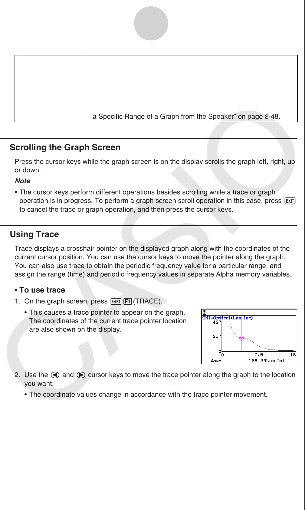
k Using Trace
Trace displays a crosshair pointer on the displayed graph along with the coordinates of the
current cursor position. You can use the cursor keys to move the pointer along the graph.
You can also use trace to obtain the periodic frequency value for a particular range, and
assign the range (time) and periodic frequency values in separate Alpha memory variables.
• To use trace
1. On the graph screen, press !1(TRACE).
• This causes a trace pointer to appear on the graph.
The coordinates of the current trace pointer location
are also shown on the display.
2. Use the d and e cursor keys to move the trace pointer along the graph to the location
you want.
• The coordinate values change in accordance with the trace pointer movement.
• You can exit the trace pointer at any time by pressing J.
• To obtain the periodic frequency value
1. Use the procedure under “To use trace” above to start a trace operation.
2. Move the trace pointer to the start point of the range whose periodic frequency you want
to obtain, and then press w.