User Manual

ε-39
Graph Analysis Tool Graph Screen Operations
12. Graph Analysis Tool Graph Screen Operations
This section explains the various operations you can perform on the graph screen after
drawing a graph.
You can perform these operations on a graph screen produced by a sampling operation,
or by the operation described under “Selecting an Analysis Mode and Drawing a Graph” on
page
ε-36.
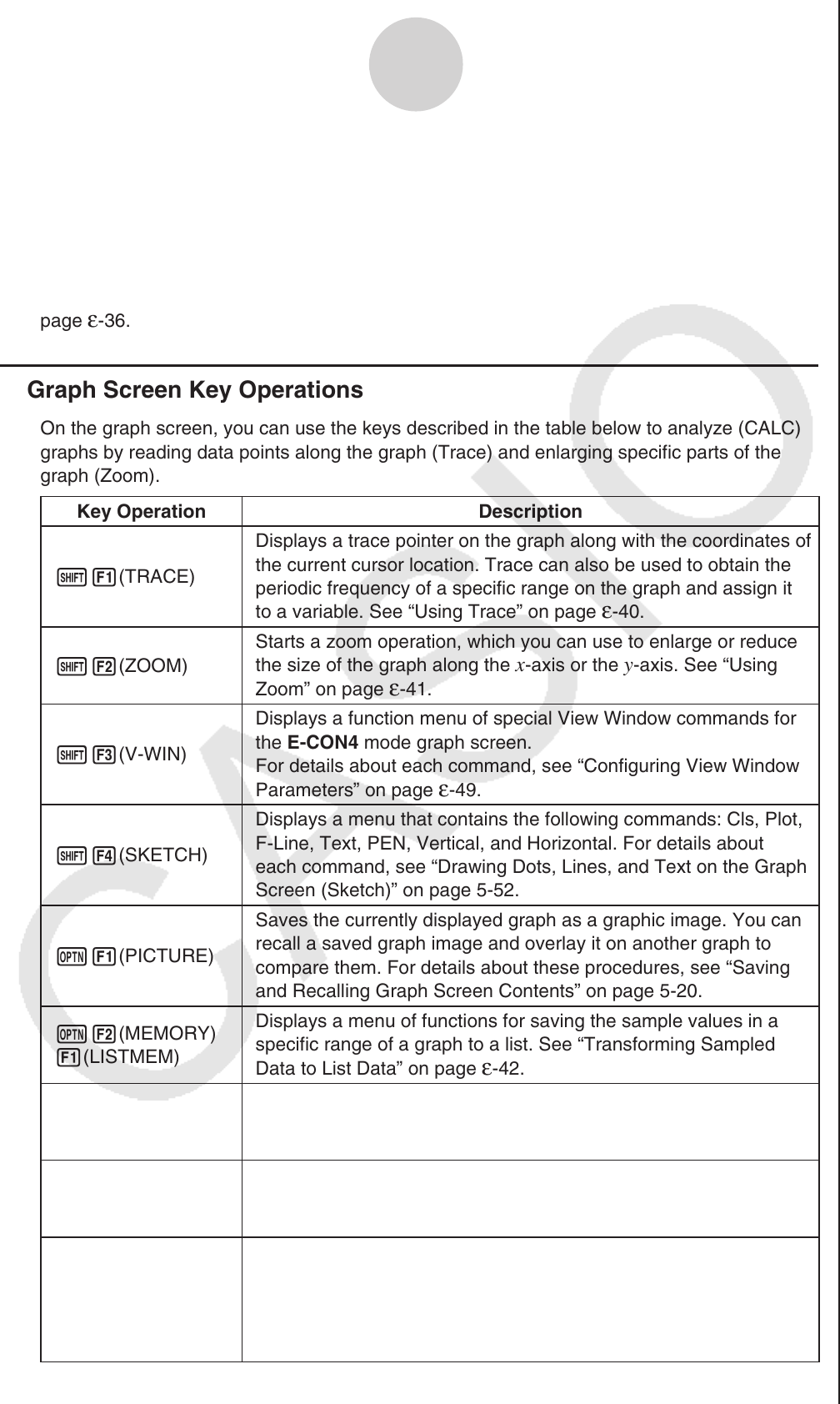
k Graph Screen Key Operations
On the graph screen, you can use the keys described in the table below to analyze (CALC)
graphs by reading data points along the graph (Trace) and enlarging specific parts of the
graph (Zoom).
Key Operation Description
!1(TRACE)
Displays a trace pointer on the graph along with the coordinates of
the current cursor location. Trace can also be used to obtain the
periodic frequency of a specific range on the graph and assign it
to a variable. See “Using Trace” on page
ε-40.
!2(ZOOM)
Starts a zoom operation, which you can use to enlarge or reduce
the size of the graph along the
x-axis or the y-axis. See “Using
Zoom” on page
ε-41.
!3(V-WIN)
Displays a function menu of special View Window commands for
the E-CON4 mode graph screen.
For details about each command, see “Configuring View Window
Parameters” on page
ε-49.
!4(SKETCH)
Displays a menu that contains the following commands: Cls, Plot,
F-Line, Text, PEN, Vertical, and Horizontal. For details about
each command, see “Drawing Dots, Lines, and Text on the Graph
Screen (Sketch)” on page 5-52.
K1(PICTURE)
Saves the currently displayed graph as a graphic image. You can
recall a saved graph image and overlay it on another graph to
compare them. For details about these procedures, see “Saving
and Recalling Graph Screen Contents” on page 5-20.
K2(MEMORY)
1(LISTMEM)
Displays a menu of functions for saving the sample values in a
specific range of a graph to a list. See “Transforming Sampled
Data to List Data” on page
ε-42.
K2(MEMORY)
2(CSV)
Saves the sample data in the specific range of a graph to a CSV
file. For details, see “Saving Sample Data to a CSV File” (page
ε-43).
K3(EDIT)
Displays a menu of functions for zooming and editing a particular
graph when the graph screen contains multiple graphs. See
“Working with Multiple Graphs” on page
ε-46.
K4(CALC)
Displays a menu that lets you transform a sample result graph to a
function using Fourier series expansion, and to perform regression
to determine the tendency of a graph. See “Using Fourier Series
Expansion to Transform a Waveform to a Function” on page
ε-44,
and “Performing Regression” on page ε-45.